Chapter1 Signals and Systems.md

Chapter1 Signals and Systems

Introduction

1. 已知输入和系统，求输出：输出预测
2. 已知输出和系统，求输入：逆向问题
3. 已知输入和输出，求系统：系统分析（与设计）

Mathmatical definition of signal

• A signal is a mathematical function that is created to transmit information.

• Function is a mathematical entity that includes

  • independent variables
  • dependent variables
  • mapping that describes their relationship

• All signals studied in this course are representable with the use of functions

Signal types

• Continuous-time signals
  • The underlying signal has a value at every point in time.
• Discrete-time signals
  • The underlying signal has values only at a discrete set of time points.

Examples:

• Continuous-time signal example:
  • speech signal $x(t)$
  • painting : continuous-time two-dimensional signal $x(t_1,t_2)$
• Discrete-time signal example
  • stock market index: discrete-time one-dimensional signal $x[n] \, n \in \mathbb{Z}$
  • Digitalized picture is a discrete-time two-dimensional signal $x[n_1,n_2]$

Signal Type	Domain	Multi-Dimensional	Value Type
Continuous-Time	Continuous	Yes (images, videos, etc.)	Real or Complex
Discrete-Time	Discrete	Yes (digitalized images, videos, etc.)	Real or Complex

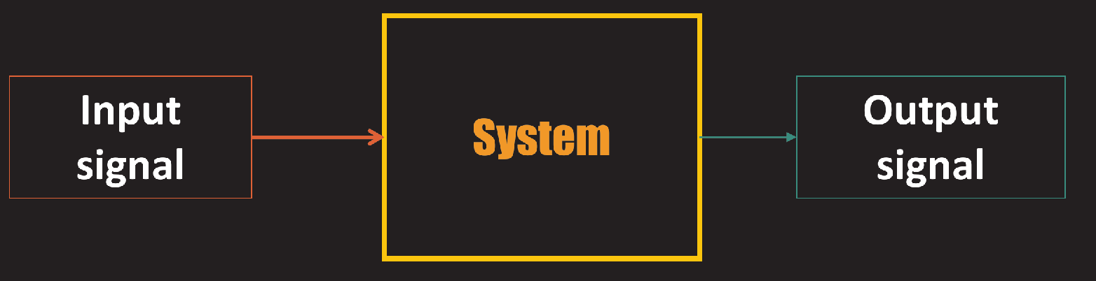
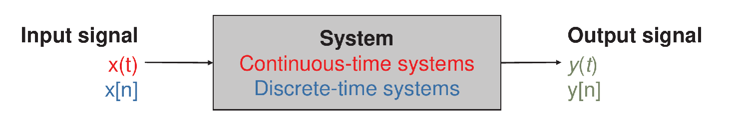
System: signal processor

• A system is a signal processor that maps a function (input signal) intoanother function (output signal)

System properties:

• Linear / non-linear
• Time-invariant / time-variant

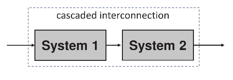
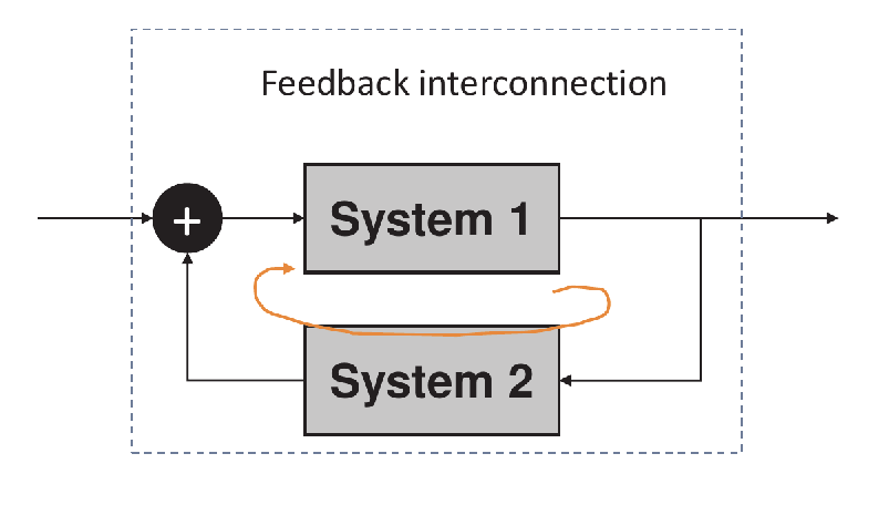
Interconnections of systems

System interconnection: connecting small systems to generate large, complicated systems

• Series (cascaded) interconnection 串联/级联

  

• Parallel interconnection 并联

  

• Feedback interconnection 反馈

  

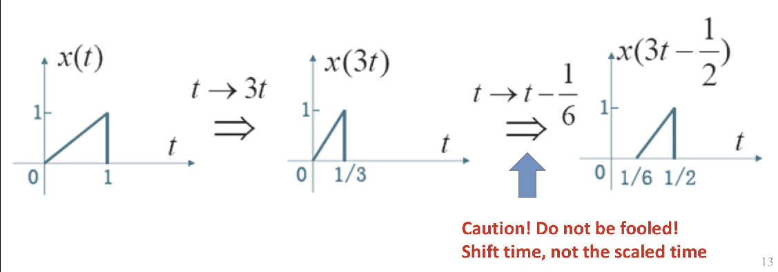
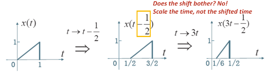
Transformations of independent variable

Time Scaling 尺度变换

$$x(t) \to x\left(\frac{t}{\alpha}\right)$$

Intuitively, this transformation squeeze or stretch the original signal

• $|\alpha| < 1$ , “Squeezing”
• $|\alpha| > 1$, “Stretching”

Important Notice: When we squeeze or stretch by applying $x(\frac{t}{\alpha})$, we squeeze
or stretch the signal about $t = 0$

Time Shifting 时移

Time Shift for continuous-time signals

$$x(t) \to x(t-t_0)$$

• $t_0 > 0$, right shift or delay the signal 延迟
• $t_0 < 0$, left shift or anti-delay the signal 提前

Time Shift for discrete-time signals

$$x[n] \to x[n-n_0], n_0 \in \mathbb{Z}$$

• You cannot always do time-scaling in the time domain for discrete-time signals because it can produce some undefined situations

Notice

• You should always scale the time ( $t$ itself ), not the shifted time !
• Identically, you should always shift the time ( $t$ itself ), not the scaled time !

Time Reversal 时间反转

$$x(t) \to x(-t)$$

Continuous-time (CT) sinusoidal signals

Definition: A sinusoidal signal is any signal whose function is derived from a standard cosine function [cos(t)] through:

1. **Magnitude scaling** (amplitude adjustment)
2. **Time scaling** (frequency adjustment)
3. **Time shifting** (phase adjustment)

$$x(t) = A \cos (\omega_0 t + \phi)$$

• A amplitude (=magnitude scaling)
• $\omega$ frequency (=time scaling)
• $\phi$ phase (=time shifting of $-\frac{\phi}{\omega_0}$)

From trigonometric identity（三角恒等式）, we know

$$\sin \theta = \cos \left(\theta - \frac{\pi}{2}\right)$$

• So sine function is just a $\frac{\pi}{2}$ phase change of cosine function
• For any magnitude, frequency, and phase, cosine and sine are identical except for a 90°phase change

Property 1: periodicity

Definition of Periodicity

• A signal $x(t)$ is periodic if and only if there exists a number $T_0$ such that:

  $$x(t) = x(t - T_0) \quad \text{for all } t$$

• The smallest such $T_0$ is called the fundamental period.

• In signal analysis, a signal $$x(t)$$ is periodic if there exists a $$T_0$$ such that the signal equals itself after a time shift of $$T_0$$.

Periodicity of Sinusoidal Signals

• A sinusoidal signal of the form:

  $$x(t) = A \cos(\omega_0 t + \phi)$$

  is periodic.

• The fundamental period of this signal is:

  $$T_0 = \frac{2\pi}{\omega_0}$$

Property 2: time-shift = phase-change

a time shift is equivalent to a phase change for a sinusoidal signal ( $\omega_0 \neq 0$ )

• Time shift $\to$ phase change
• Phase change $\to$ time shift
• An indication: sine is cosine shifted by a quarter (1/4) of a period $\frac{T}{4}$

Proof

$$y(t) = A \cos (\omega_0 (t-t_0) + \phi) = A \cos (\omega_0 t - \omega_0 t_0 + \phi)$$

So Let $\Delta \phi = -\omega_0 t_0$, then

$$y(t) = A \cos (\omega_0 t + \phi + \Delta \phi)$$

Identically,

$$y(t) = A(\omega_0 t + \phi + \Delta \phi) = A(\omega_0(t + \frac{\Delta \phi}{\omega_0}) + \phi)$$

So Let $\Delta t = -\frac{\Delta \phi}{\omega_0}$, then

$$y(t) = A\cos(\omega_0 (t-\Delta t) + \phi)$$

Property 3: symmetry of sinusoidal signals

Definition

Even Symmetry

• A signal is even iff

$$x(t) = x(-t)$$

• Symmetric about the y-axis

Odd Symmetry

• A signal is odd iff

$$x(t) = -x(-t)$$

• Anti-symmetric, or symmetric about the point of origin

Even & odd decomposition

• Any real-valued signal can be decomposed into a sum of an even signal and odd signal

• To see it, define:

  $$x_e(t) = \mathcal{Ev} \{x(t)\} \triangleq \frac{1}{2} \left[ x(t) + x(-t) \right] \\ x_o(t) = \mathcal{Od} \{x(t)\} \triangleq \frac{1}{2} \left[ x(t) - x(-t) \right]$$

• The original signal can be expressed as:

  $$x(t) = x_e(t) + x_o(t)$$

  • Here: $x_e(t)$ is the even component of the signal, $x_o(t)$ is the odd component of the signal.

• Any real-valued signal can be decomposed into its even and odd components, as defined above.

CT real exponential

$$x(t) = C e^{\alpha t} , C \in \mathbb{R}, \alpha \in \mathbb{R}$$

• Assume $$C > 0$$

  • a > 0$$: The exponential is **growing**.

  • a = 0$$: The exponential is a **constant** ($$x(t) = C$$).

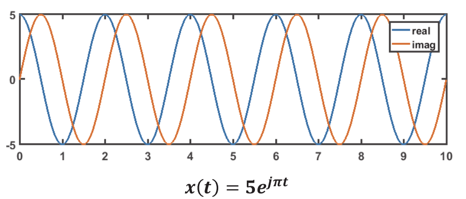
• Polar form（极坐标形式） of CT complex exponential signal

$$x(t) = C e^{\alpha t}, C \in \mathbb{C}, \alpha \in \mathbb{C}$$

• The rectangular/Cartesian form（直角坐标/笛卡尔形式） of complex exponential signal
  • let $C = |C| e^{j \phi}, \alpha = \gamma + j \omega_0$

$$x(t) = |C| e^{\gamma t}\cos (\omega_0 t + \phi) + j |C| e^{\gamma t}\sin (\omega_0 t + \phi)$$

• Both the real and imaginary parts are:
  • sinusoidal signals with a time-varying amplitude $|C|e^{\gamma t}$ (envelope 包络线)
  • This highlights the relationship between sinusoidal and exponentials

A special case

• If $$Re{a} = \gamma = 0$$, then

$$x(t) = |C| \cos(\omega_0 t + \phi) + j|C| \sin(\omega_0 t + \phi)$$

• Both real and imaginary part are pure sinusoidal signals

Signal decomposition

• Almost all real signals can be represented by linear combinations of sinusoidal signals

  $$x(t) = \sum_{n=0}^{\infty} A_n \cos(\omega_n t + \theta_n), \quad x(t), A_n \in \mathbb{R}$$

• Almost all complex signals can be represented by linear combinations of complex exponential signals

  $$x(t) = \sum_{n=-\infty}^{\infty} C_n e^{j\omega_n t}, \quad x(t), C_n \in \mathbb{C}$$

Discrete-time (DT) sinusoidal signals

• DT signals are just sampled CT signals
• Definitions and properties of DT signals are generally similar to CT signals.
• However, the discretization process can lead to the loss of certain properties inherent in the original CT signals.

DT sinusoidal

Definition

$$x[n] = A \cos (\Omega_0 n + \phi), n \in \mathbb{Z}$$

• Where:

  • A$$: Amplitude

  • \phi$$: Phase

lost property #1

• Phase change $\nRightarrow$ time shift (Reverse still holds)
• Time shift $\implies$ phase change
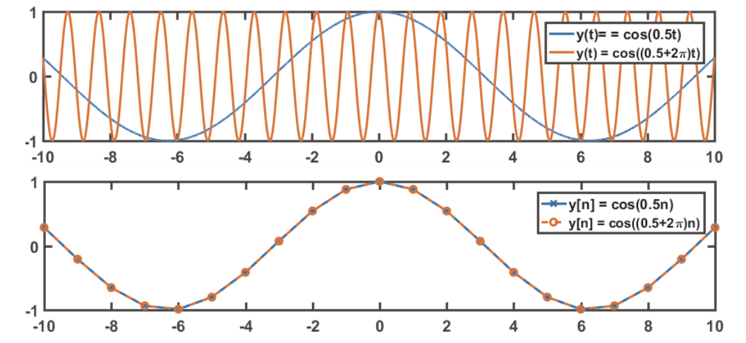
• The key point is that in DT signals, any time shift must be an integer. If the ratio of phase change and frequency $-\frac{\Delta \phi}{\omega_0}$ is not an integer, the phase change does not imply a time shift.

lost property #2

• DT sinusoidal is not necessarily periodic
• In general, DT sinusoidal is periodic iff $\frac{2\pi}{\Omega_0}$ (the period of its CT version) is a rational number.
  • When a DT sinusoidal signal is periodic, its fundamental period $$p$$ is the smallest positive integer such that $$\frac{2\pi}{\Omega_0} = \frac{p}{q}$$, where $$p$$ and $$q$$ are coprime integers (i.e., their greatest common divisor is 1).

lost property #3

• Different frequencies do not imply different signals
• This is because: $$A\cos(\Omega_0 n + \phi) = A\cos((\Omega_0 + 2\pi m)n + \phi)$$ if $$\Omega_1 - \Omega_0 = 2\pi m$$ for any integer $$m$$.
• 这就是将连续信号采样为离散信号时会出现混叠的原因

DT exponential

• Real exponentialc

• Complex exponential (by default)

• DT sinusoidal signals are building blocks of DT real signals

• DT Complex exponential signals are building blocks of DT complex signals

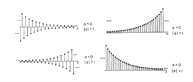
DT real exponential

1. Algebraic Definition:

   $$x[n] = C a^n$$

   • $C$ and $a$ are real numbers ($C \in \mathbb{R}$, $a \in \mathbb{R}$, $n \in \mathbb{Z}$).
   • Note: This is not a direct sampling of the CT exponential ($Ce^{\beta t}$).

2. Relationship to CT Real Exponential Signal:

   • Case 1: If $a > 0$, there exists $\beta \in \mathbb{R}$ such that $a = e^{\beta}$, and the DT signal becomes: $$x[n] = C e^{\beta n}$$
     • This is a sampling of the CT real exponential.
   • Case 2: If $a < 0$, the DT real exponential is not a direct sampling of the CT real exponential.

3. Behavior of $C a^n$:

   • Decaying Signal: If $|a| < 1$, the signal decays as $n$ increases.
   • Growing Signal: If $|a| > 1$, the signal grows as $n$ increases.
   • Oscillatory Signal: If $a < 0$, the signal alternates in sign.

4. Advantage of DT Real Exponential:

   • The form $C a^n$ increases the range of signals that can be represented by discrete-time real exponentials compared to CT exponentials.

DT Complex Exponential:

Algebraic Definition

• Polar Form:

  $$x[n] = C a^n$$

  • $C$ and $a$ are complex numbers ($C \in \mathbb{C}$, $a \in \mathbb{C}$).

• Rectangular Form:
  Let $C = |C|e^{j\phi}$ and $a = |a|e^{j\Omega_0}$, then:

  $$x[n] = |C||a|^n \cos(\Omega_0 n + \phi) + j|C||a|^n \sin(\Omega_0 n + \phi)$$

• This represents the real and imaginary parts of the DT complex exponential.

Behavior of DT Complex Exponential

• Magnitude of $a$:
  • If $|a| > 1$, the signal grows exponentially.
  • If $|a| < 1$, the signal decays exponentially.
• Frequency $\Omega_0$: Determines the oscillation frequency of the signal.

Relationship to CT Complex Exponential

• DT complex exponentials are direct samplings of CT complex exponential signals.
• However, the real and imaginary parts of the DT signal are not necessarily related by a time shift (unlike CT signals).

Envelope of the Signal

• The envelope of the signal is determined by $|C||a|^n$:
  • If $|a| > 1$, the envelope grows exponentially.
  • If $|a| < 1$, the envelope decays exponentially.

Visual Representation

• The signal can be visualized as a combination of growing/decaying oscillations (real and imaginary parts) modulated by the envelope $|C||a|^n$.

Signal Energy and Power

Finite Time Interval

Energy

• The total energy of a signal over a finite time interval is defined by (CT or DT):

  $$E = \int_{t_1}^{t_2} |x(t)|^2 \, dt \quad \text{(Continuous Time)}$$

  $$E = \sum_{n=n_1}^{n_2} |x[n]|^2 \quad \text{(Discrete Time)}$$

• If $x(t)$ is real-valued, $| x(t) |$ is the absolute value.

• If $x(t)$ is complex-valued, $| x(t) |$ is the magnitude.

  • $|x(t)|^2 = x(t) x^*(t)$

Average Power (P)

• The average power $P$ over a time interval is defined based on the energy $E$ of the same time interval divided by the length of the interval:

  $$P = \frac{E}{t_2 - t_1} \quad \text{(Continuous Time)}$$

  $$P = \frac{E}{n_2 - n_1 + 1} \quad \text{(Discrete Time)}$$

Entire Time Domain

Energy

• The total energy of a signal over the entire time domain is defined by (CT or DT):

  $$E_\infty = \int_{-\infty}^{\infty} |x(t)|^2 \, dt \quad \text{(Continuous Time)}$$

  $$E_\infty = \sum_{n=-\infty}^{\infty} |x[n]|^2 \quad \text{(Discrete Time)}$$

• If $x(t)$ is real-valued, $| \cdot |$ is the absolute value.

• If $x(t)$ is complex-valued, $| \cdot |$ is the magnitude.

  • $|x(t)|^2 = x(t) x^*(t)$

Average Power

• The average power over the entire time domain is:

  $$P_\infty = \lim_{T \to \infty} \frac{1}{2T} \int_{-T}^{T} |x(t)|^2 \, dt \quad \text{(Continuous Time)}$$

  $$P_\infty = \lim_{N \to \infty} \frac{1}{2N+1} \sum_{n=-N}^{N} |x[n]|^2 \quad \text{(Discrete Time)}$$

Three Types of Signals

1. Signals with Finite Total Energy Over the Entire Time Domain

   • Example:

     $$x(t) = \begin{cases} 1 & \text{for } 0 < t < 1 \\ 0 & \text{otherwise} \end{cases}$$

   • Total Energy $E_\infty = 1$

   • Average Power $P_\infty = 0$

2. Signals with Finite Average Power Over the Entire Time Domain

   • Example:

     $$x[n] = 1 \quad \text{for all } n$$

   • Average Power $P_\infty = 1$

   • Total Energy $E_\infty = \infty$

3. Signals with Infinite Energy and Power Over the Entire Time Domain

   • Example:

     $$x(t) = t$$

   • Both Total Energy $E_\infty = \infty$ and Average Power $P_\infty = \infty$

Properties of energy

• Energy does not care sign of the signal; it exists no matter the signal is positive or negative.
• Energy is also invariant under time shift and time reversal, but it changes under time scaling

Some thoughts and conclusions

• Discrete-Time Signals: Zero energy $\implies$ signal is zero everywhere.
• Continuous-Time Signals: Zero energy does not imply the signal is zero everywhere, as the signal can be non-zero at isolated points or over intervals of zero measure. (e.g., a finite number of points or a set with zero length)

Signal algebra

Signal manipulations by y-axis operations

Signal addition

$$f[n] = x[n] + y[n] \, \text{or} \, f(t) = x(t) + y(t)$$

Multiplication/division

multiply/divide at every time point

$$f[n] = x[n] \times y[n]\, \text{or}\, f(t)=x(t) \times y(t)$$

Continuous: First-order derivative of continuous-time signals

$$y(t) = \frac{d x(t)}{dt} = x'(t)$$

Continuous: Running integral of continuous-time signals

$$y(t) = \int_{\infty}^{t} x(\tau) \, d\tau$$

x(t) is the first-order derivative of y(t)

Discrete: First-order difference/first difference

$$y[n] = x[n] - x[n-1]$$

Discrete: Running sum of discrete-time signal

$$y[n] = \sum_{k=-\infty}^{n} x[k]$$

Note that x[n] is the first difference of y[n]

If you firstly take finite difference, and then running sum, do you necessarily get back the same signal?

NO! Beacuse the constant component (DC component) will be removed!

Basic Signals

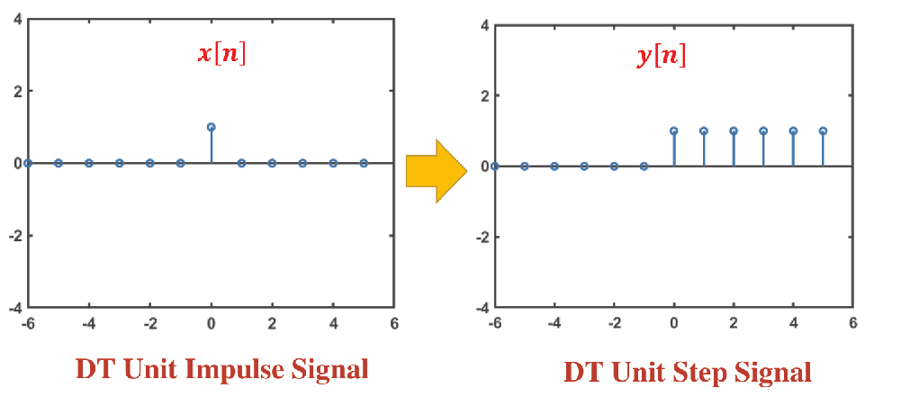
Unit Step & Unit Impulse

they are commonly used testing signals

DT unit step & unit impulse

Definition

$$u[n] = \begin{cases} 1 & n \geq 0 \\ 0 & n < 0 \end{cases}$$

Notations for unit step signal: $u[n]$ or $u(t)$

$$\delta [n] = \begin{cases} 1 & n = 0\\ 0 & n \neq 0 \end{cases}$$

Notations for unit impulse signal: $\delta [n]$ or $\delta (t)$

Properties:

• unit impulse is the first difference of unit step
• unit step is running sum of unit impulse

$$\delta[n] = u[n] - u[n-1] \\ u[n] = \sum_{k=-\infty}^n \delta[k]$$

CT unit step & unit impulse

Definition

CT unit step

$$u(t) = \begin{cases} 1 & t \geq 0 \\ 0 & t < 0 \end{cases}$$

CT unit impulse

$$\delta(t) = \begin{cases} +\infty & t = 0 \\ 0 & t \neq 0 \end{cases}$$

This is somewhat ill-defined!

So the best mathmatical definition is to use auxiliary functions

$$u_{\Delta}(t) = \begin{cases} 0 & t < 0 \\ \frac{t}{\Delta} & 0 \leq t < \Delta \\ 1 & t \geq \Delta \end{cases} \quad \delta_{\Delta}(t) = \begin{cases} \frac{1}{\Delta} & 0 < t \leq \Delta \\ 0 & \text{otherwise} \end{cases}$$

Then use the limit-of-convergence definition

$$u(t) = \lim_{\Delta \to 0} u_{\Delta} (t) \quad \delta(t) = \lim_{\Delta \to 0} \delta_{\Delta} (t)$$

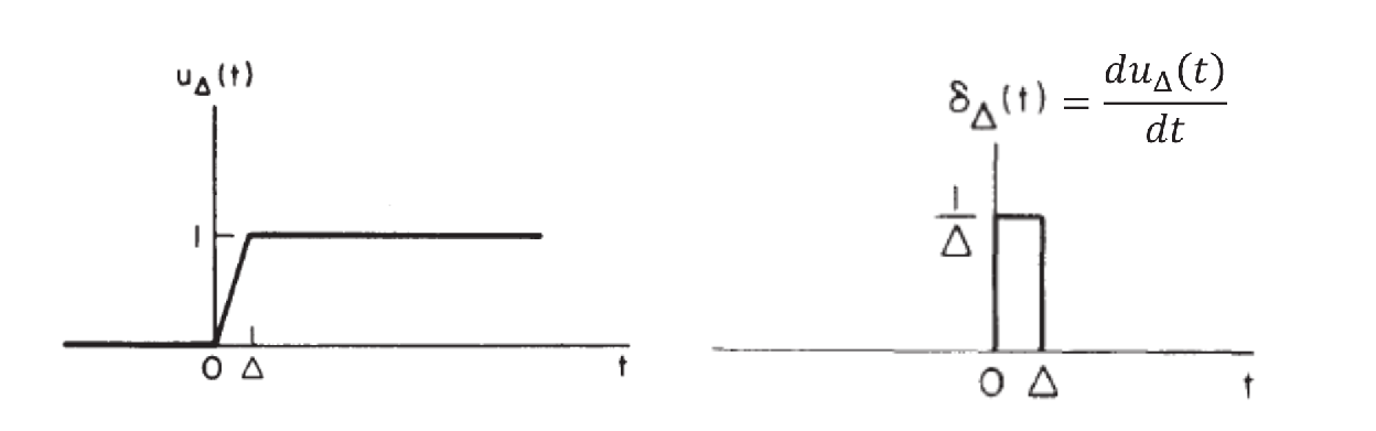
• The limit-of-convergence definition ensures that the derivative-integration relationship between the unit step and unit impulse functions, by ensuring the relationship holds for $u_\Delta (t)$ and $\delta_\Delta (t)$ every $\Delta$.
• CT unit impulse has “zero width, infinite height, and area 1”.
• Graphical representation:

In conclusion, we have some good properties:

$$\delta(t) = \frac{d u(t)}{dt} \quad u(t) = \int_{-\infty}^t \delta (t) \, dt$$

Example questions

$$x[n] = \sum_{k=-\infty}^\infty \delta[n-4k]$$

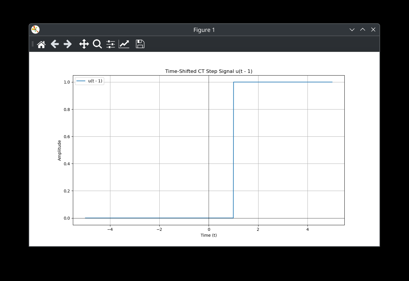
The result is an impulse train signal

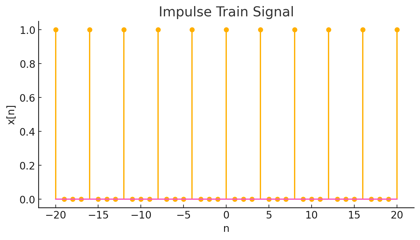$$ x(t) = \int_{-\infty}^t \delta(\tau - 1)d\tau $$ The result is a time shifted CT step signal $$ x(t) = u(t-1) $$

Description of systems

System Equations

• System is often described by an equation that links each input to its corresponding output.

• These equations can be simple; in this case we have a simple system. Some examples are:

  • Time-shifting system: $y(t) = x(t - T)$ or $y[n] = x[n - N]$
  • Time-scaling system: $y(t) = x(at)$ or $y[n] = x[an]$
  • Squarer: $y(t) = (x(t))^2$ or $y[n] = (x[n])^2$
  • Differentiator: $y(t) = \frac{dx(t)}{dt}$ or $y[n] = x[n] - x[n - 1]$
  • Integrator: $y(t) = \int_{-\infty}^t x(\tau)d\tau$ or $y[n] = \sum_{k=-\infty}^n x[k]$

Order of system interconnections

• Series interconnection: In general, a reversely ordered series interconnection changes the original system.
• Parallel interconnection: order does not matter
• Feedback interconnection: order of course matters

System Properties

• we often describe the system by system properties, which are partial knowledge about the input-output relationship.
• Major properties include:
  • Memoryless (Time-dependent)
  • Causality (Time-dependent)
  • Invertibility (Time-independent)
  • Stability (Time-independent)
  • Linearity (Time-independent)
  • Time-invariance (Time-independent)

Time-dependent vs time-independent

• Time-dependent properties only considers how system behaves along the time dimension
• Time-independent properties only considers how system behaves along the signal dimension

Memoryless property

• Definition: the value of output at any time point is only dependent on the value of input at the same time point.
• Definition in a mathematical form:

$y(t)|_{t=t_0} \text{ is only dependent on } x(t)|_{t=t_0} \text{ for every } x(t)$

$y[n]|_{n=n_0} \text{ is only dependent on } x[n]|_{n=n_0} \text{ for every } x[n]$

Causality

1. Definition: A system is causal if the output at any given time point depends only on the input at or before that same time point. In other words, the system does not rely on future inputs to produce its current output.

2. Mathematical Formulation:

   • For continuous-time systems:

     y(t) \big|_{t=t_0} $$ depends only on $$ x(t) \big|_{t \leq t_0} $$ for every input $ x(t) $.

     y[n] \big|_{n=n_0} $$ depends only on $$ x[n] \big|_{n \leq n_0} $$ for every input $ x[n] $.

   • A memoryless system (where the output at any time depends only on the input at that same time) is always causal.
   • However, the converse is not true: A causal system is not necessarily memoryless. Causal systems can have memory (depend on past inputs).

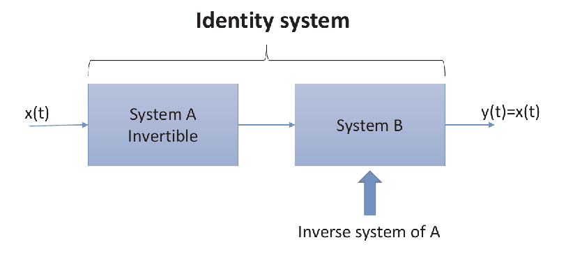
Invertibility

• Definition for invertible system: there is only one input signal for every output signal
• Alternative definition: different input signals lead to different output signals

Inverse system and identity system

• For an invertible system, its inverse system is defined as the system mapping each output of the original system to its corresponding input.
  • For example, if A is an running sum system, then B is an first difference system.
• Cascading a system and its inverse system forms an identity system

Stability 稳定性

1. Definition of Stability: A system is considered stable if it satisfies the BIBO (Bounded Input Bounded Output) condition. This means that for any bounded input, the output remains bounded.

2. Boundedness:

   • An input $x(t)$ is bounded if there exists a positive number $m$ such that: $$ |x(t)| < m $$ for all $t$.
   • Similarly, the output $y(t)$ must also remain bounded for the system to be stable.

3. BIBO Stability:

   • A system is BIBO stable if and only if for any bounded input, the output is also bounded.
     • To prove BIBO stable, we need to show for an arbitrary bounded input, the output is also bounded
   • Mathematically, if $|x(t)| < m$ for all $t$, then there exists a positive number $M$ such that: $$ |y(t)| < M $$ for all $t$.

4. Unstable Systems:

   • A system is unstable if there exists at least one bounded input that produces an unbounded output.
     • To prove unstability, we need only one bounded input that generates unbounded output. (One counter-example is enough.)

System Properties

Linearity 线性

Definition of Linearity in a System:

A system is linear if, for any two inputs $x_1(t)$ and $x_2(t)$ producing outputs [y_1(t)] and [y_2(t)], the following two conditions are satisfied:

1. Additivity Property: 可加性

   $$x_1(t) + x_2(t) \to y_1(t) + y_2(t)$$

2. Homogeneity Property: 齐次性

   $$a x_1(t) \to a y_1(t) \quad \text{for any complex number } a$$

Partial Knowledge Gained from Linearity:

1. If we know the responses of two individual signals, we can determine the response of their sum.
2. If we know the response of a single signal, we can determine the response of that signal after any rescaling.

Proof or disproof

• To prove a system is linear, we need to show for any input signal(s), both the additivity and homogeneity hold.
• On the other hand, to prove a system is nonlinear, we need to show there exist some input signal(s), for which either the additivity or homogeneity does not hold.

Simplified definition for linearity(更常用)

A system is linear iff

$$a_1x_1(t) + a_2x_2(t) \rightarrow a_1y_1(t) + a_2y_2(t)$$

for any inputs $x_1(t)$, $x_2(t)$, and any complex numbers $a_1$ and $a_2$.

Generalization of Linearity

1. Concept:

   • Linearity can be extended to any number of input signals.
   • If a system is linear, then for any positive integer $K$ , the following holds:

   $$\sum_{k=1}^{K} a_k x_k(t) \rightarrow \sum_{k=1}^{K} a_k y_k(t)$$

   Here, $x_k(t)$ are the input signals, $y_k(t)$ are the corresponding outputs, and $a_k$ are complex coefficients.

2. Key Insight: The response of a linear system to a linear combination of input signals is the same linear combination of their individual outputs.

Quick Ruling-Out of Linearity

1. Zero-In Zero-Out (ZIZO) Property
   • If a system is linear, it must satisfy: If $x(t) = 0$ for all $t$, then $y(t) = 0$ for all $t$.
2. Proof: Uses homogeneity
   • $0 = 0 \cdot a(t) \to 0 \cdot b(t) = 0$, where $a(t)$ is an arbitrary signal and $b(t)$ is its response.
3. Necessary but Not Sufficient: ZIZO is a necessary condition for linearity, but not sufficient (e.g., a squarer satisfies ZIZO but is not linear).

Time-invariance 时不变性

1. Definition: For any time-shift $t_0$ (for CT systems) or $n_0$ (for DT systems) and any input signal $x(\cdot)$:

   • Continuous-Time (CT) System:

     $$x(t - t_0) \rightarrow y(t - t_0)$$

   • Discrete-Time (DT) System:

     $$x[n - n_0] \rightarrow y[n - n_0]$$

2. Key Insight: A time shift in the input signal causes no change in the output except for an identical time shift.

解题方法

线性与时不变性的证明思路

• Proof of linearity
  • Evaluating output of $a_1 x_1(t) + a_2 x(t)$
  • Evaluating $a_1 y_1(t) + a_2 y_2(t)$
  • If equal $\implies$ linear system
• Proof of Time-invariance
  • Evaluating output of $x(t - t_0)$
  • Evaluating $y(t-t_0)$
  • If equal $\implies$ time-invariance

Template

1. Proving Linearity

   1. Define Inputs and Scalars: Let $$ x_1(t) $$, $$ x_2(t) $$ be input signals, and $$ a_1 $$, $$ a_2 $$ be complex numbers.
   2. Apply Superposition to Input: Let $$ w(t) = a_1x_1(t) + a_2x_2(t) $$.
   3. Evaluate System Response to Superposition: Compute $$ z(t) = \text{System}{w(t)}$$.
   4. Evaluate Superposition of Output: On the other hand, Compute $$y(t) = a_1y_1(t) + a_2y_2(t)$$, where $$ y_i(t) = \text{System}{x_i(t)} $$.
   5. Compare result of 3 and 4: Verify if $$ z(t) = a_1y_1(t) + a_2y_2(t)$$
   6. Conclusion: If equal, the system is linear; otherwise, it’s nonlinear.

2. Proving Time-Invariance

   1. Define Input and Time Shift: Let $$ x(t) $$ be an input signal and $$ T_0 $$ be a time shift.
   2. Apply Time Shift to Input: Let $$ w(t) = x(t - T_0) $$.
   3. Evaluate System Response to Shifted Input: Compute $$ z(t) = \text{System}{w(t)} $$.
   4. Evaluate Shifted Output: On the other hand, Compute $$y(t - T_0)$$, where $$ y(t) = \text{System}{x(t)} $$.
   5. Compare with Shifted Output: Verify if $$ z(t) = y(t - T_0) $$
   6. Conclusion: If equal, the system is time-invariant; otherwise, it’s time-variant

附录：数学知识补充

Triangle Inequality 三角不等式

$$|x_1(t) + x_2(t)| \leq |x_1(t)| + |x_2(t)|$$

At the same time,

$$\left| |x_1(t)| - |x_2(t)| \right| \leq |x_1(t) - x_2(t)|$$