Chapter2 LTI Systems

Linear Time-Invariant (LTI) Systems

Definition

• An LTI system is both linear and time-invariant.

Key Properties

1. Input-Output Relationship:

• For a Continuous-Time (CT) LTI system:

  $$\sum_{k=1}^{K} a_k x_k(t - t_k) \rightarrow \sum_{k=1}^{K} a_k y_k(t - t_k)$$

  • This holds for any input $x_k(t)$, delay $t_k$, weight $a_k$, and positive integer $K$.
• For a Discrete-Time (DT) LTI system:

  $$\sum_{k=1}^{K} a_k x_k[n - n_k] \rightarrow \sum_{k=1}^{K} a_k y_k[n - n_k]$$

  • This holds for any input $x_k[n]$, delay $n_k$, weight $a_k$, and positive integer $K$.

2. Impulse Response and Convolution:
   • The output of an LTI system can be predicted using convolution.
   • The key idea is to represent any input signal as a linear combination of time-shifted impulses.
   • The system’s response to an impulse (impulse response) fully characterizes the system.

Implications

• The response of an LTI system to a linear combination of time-shifted inputs is the same linear combination of the identically shifted original outputs.
• This property simplifies the analysis and prediction of system behavior, making convolution a fundamental tool for studying LTI systems.

Convolution representation of LTI systems

Unit Impulse Representation of Discrete-Time (DT) Signals

Key Concepts

1. Unit Impulse Representation:

   • The discrete-time signal $$x[n]$$ can be represented as a sum of weighted, shifted unit impulses:

     $$x[n] = \sum_{k=-\infty}^{\infty} x[k] \delta[n - k]$$

   • Here, $$\delta[n - k]$$ is the unit impulse function.

2. Unit Impulse Response:

   • Let $$h[n]$$ represent the unit impulse response:

     $$\delta[n] \rightarrow h[n]$$

3. Linearity and Time-Invariance (LTI) Property:

   • For an LTI system, the response to a linear combination of shifted impulses is the same linear combination of the corresponding shifted impulse responses:

     $$\sum_{k=-\infty}^{\infty} \alpha_k \delta[n - n_k] \rightarrow \sum_{k=-\infty}^{\infty} \alpha_k h[n - n_k]$$

4. Convolution Sum:

   • Applying the LTI property to the representation of $$x[n]$$, we get:

     $$x[n] = \sum_{k=-\infty}^{\infty} x[k] \delta[n - k] \rightarrow \sum_{k=-\infty}^{\infty} x[k] h[n - k]$$

   • This is known as the convolution sum between $$x[n]$$ and $$h[n]$$, which is a linear combination of shifted impulse responses.

Conclusion

• The convolution sum describes how the output of an LTI system is the weighted sum of the system’s responses to individual shifted impulses.

Convolution Representation of DT LTI Systems

1. Convolution Sum Representation
   The output $$y[n]$$ of a Discrete-Time Linear Time-Invariant (DT LTI) system can be expressed as:

   $$y[n] = \sum_{k=-\infty}^{\infty} x[k]h[n - k] = x[n] * h[n]$$

   • Here, $$x[n]$$ is the input signal.

   • h[n]$$ is the system's unit impulse response.

2. Interpretation of Convolution

   • The response of a DT LTI system to any input $$x[n]$$ is equal to the convolution of the input with the system’s unit impulse response $$h[n]$$.
   • This means the system’s behavior is fully characterized by its impulse response.

3. Intrinsic Nature of Convolution

   • The convolution sum is essentially a sum of weighted, shifted impulse responses ($$x[k]h[n - k]$$).
   • Each term corresponds to a weighted, shifted impulse ($$x[k]\delta[n - k]$$).
   • Despite this, the convolution expression does not explicitly involve unit-impulse decomposition.

Unit Impulse Representation of Continuous-Time (CT) Signals

Concept Overview

• A continuous-time (CT) signal can be approximated by a sequence of rectangular functions $\delta_\Delta(t)$.
• As $\Delta \to 0$, these rectangular approximations approach the Dirac delta function $\delta(t)$.

Approximation of CT Signal

A CT signal $x(t)$ can be approximated as:

$$x(t) \approx \sum_{k=-\infty}^{\infty} x(k\Delta) \delta_\Delta(t - k\Delta)\Delta$$

Impulse Response and LTI Systems

Impulse Response Definition

• Let $h_\Delta(t)$ be the system’s response to $\delta_\Delta(t)$.
• The impulse response $h(t)$ of the system is defined as:

  $$h(t) \triangleq \lim_{\Delta \to 0} h_\Delta(t)$$

• Thus, $h(t)$ is the system’s response to the ideal delta function $\delta(t)$.

Representation Using Convolution (For LTI Systems)

Step 1: Use Approximate Delta

$$\sum_{k=-\infty}^{\infty} x(k\Delta) \delta_\Delta(t - k\Delta) \Delta \rightarrow \sum_{k=-\infty}^{\infty} x(k\Delta) h_\Delta(t - k\Delta) \Delta$$

Step 2: Take the Limit as $\Delta \to 0$

$$\lim_{\Delta \to 0} \sum_{k=-\infty}^{\infty} x(k\Delta) h_\Delta(t - k\Delta) \Delta \rightarrow \int_{-\infty}^{+\infty} x(\tau) h(t - \tau) d\tau$$

Final Convolution Integral Representation

• The signal $x(t)$ can be expressed as:

  $$x(t) = \int_{-\infty}^{+\infty} x(\tau) \delta(t - \tau) d\tau \rightarrow \int_{-\infty}^{+\infty} x(\tau) h(t - \tau) d\tau$$

• This is the convolution integral between $x(t)$ and $h(t)$.

Convolution Representation of CT LTI Systems

• The convolution integral:

  $$\int_{-\infty}^{+\infty} x(\tau) h(t - \tau) d\tau$$

  is used to compute the output of a CT LTI system.

Key Insight

The response of a CT LTI system to any input is equal to the convolution integral of the input with the system’s unit impulse response.

• While the convolution expression does not explicitly show the unit impulse decomposition, it implicitly relies on it.

Interpretation

• The convolution integral is essentially a sum of weighted, shifted impulse responses:
  • $[x(\tau) d\tau] h(t - \tau)$: weighted response to shifted impulse.
  • $[x(\tau) d\tau] \delta(t - \tau)$: representation of $x(t)$ as an impulse-weighted sum.

Definition of Convolution

Convolution is a fundamental operation in signal processing and linear systems, used to express the output of a system in terms of its input and its impulse response.

🔹 Discrete-Time Convolution (Convolution Sum)

For discrete-time signals $x[n]$ and $h[n]$, the output $y[n]$ is given by:

$$y[n] = \sum_{k=-\infty}^{+\infty} x[k] \cdot h[n - k] = x[n] * h[n]$$

This is called the convolution sum.

🔹 Continuous-Time Convolution (Convolution Integral)

For continuous-time signals $x(t)$ and $h(t)$, the output $y(t)$ is given by:

$$y(t) = \int_{-\infty}^{+\infty} x(\tau) \cdot h(t - \tau) \, d\tau = x(t) * h(t)$$

This is called the convolution integral.

Convolution with Unit Impulse

• $x(t) * \delta(t) = \int_{-\infty}^{\infty} x(\tau) \delta(t - \tau) \, d\tau$

  • Since $$ \delta(t - \tau) = 0 $$ except at $$ \tau = t $$, it follows:

  • $$\int_{-\infty}^{\infty} x(t) \delta(t - \tau) \, d\tau = x(t) \int_{-\infty}^{\infty} \delta(t - \tau) \, d\tau = x(t)$$

• Thus:

  $$x(t) * \delta(t) = x(t) \quad \text{(unit impulse convolving with any signal returns the signal itself)}$$

• A generalized form of this property is called the convolution property of unit impulse:

  $$x(t) * \delta(t - t_0) = x(t - t_0)$$

• The identity:

  $$x(\tau) \delta(t - \tau) = x(t) \delta(t - \tau)$$

  is called the sifting property (筛选性质) of the unit impulse.

Implementation of convolutional calculations

• The implementation of convolution sum follows a “reversal-shifting-multiplication-sum” RSMS procedure.

RSMS Procedure for DT convolution sum

Goal: Compute convolution:

$$y[n] = \sum_{k=-\infty}^{\infty} x[k] h[n - k]$$

Key Steps (for fixed $n = n_0$)

1. Reverse: $h[k] \rightarrow h[-k]$
2. Shift: $h[-k] \rightarrow h[n_0 - k]$
3. Multiply: $x[k] \cdot h[n_0 - k]$
4. Sum: Over all $k$, to get $y[n_0]$

Repeat by increasing $n_0$.

For Finite Support Signals

• $y[n] = 0$ when $x[k]$ and $h[n-k]$ don’t overlap

• As $n$ increases, overlap grows, peaks, then diminishes

• Total nonzero $y[n]$:

$$\text{length}(x[k]) + \text{length}(h[k]) - 1$$

更实际的解题方法

实际情况下，卷积一般用来处理有限长度（只在有限长度区域内非零）的离散时间信号。利用这一点，使用以下的步骤解题会比较好：

1. 按照卷积的定义式子，把题目所给的信号和冲激响应代入
   • 有时候算卷积的题目就只给两个函数，要不会说哪个是信号哪个是冲激响应，那么选择比较简单的函数或者看起来比较像是系统冲激响应的那个函数作为$h[n-k]$那一边，因为后续要进行变换，这步的选择会影响后续的计算量
2. 因为基本上给你的函数是有限长度的，那么可以先判定使得$x[k]$和$h[n-k]$非零的 $k$ 的范围。若$h[k]$是分段函数，还需考虑$h[n-k]$的各分段对应的 $k$ 的范围。
   • 注意：卷积和的自变量是 $k$ ，所以这里算的是 $k$ 的范围，而这个范围的上下限可能是含有 $n$ 的表达式
   • 如果 $h[n-k]$ 是比较复杂，在这一步考虑写出其变换后的分段表达式
3. 只有$x[k]$和$h[n-k]$都非零时，卷积的值非零，其他情况卷积都是零。利用这一特性，只需计算两者都非零区间内的卷积和即可
   • 这一步需要对于 $n$ 的值在不同区域内时，两种非零范围的不同重叠情况，进行分类讨论
   • 对于分段函数，还需要考虑每个分段的重叠情况，进行更细致的分类讨论。如果太复杂，考虑画出 $h[n-k]$ 的图像来辅助判断
   • 使 $x[k]$和$h[n-k]$非零的 $k$ 的范围中含有 $n$，所以重叠情况是由 $n$ 的取值决定的，这里分类讨论的是 $n$ ！
4. 综合各种情况，得到结果

另外，

• 如果直接算搞不清楚的，可以画图辅助

RSMI Procedure for CT convolution integral

Goal:
Compute continuous-time convolution:

$$y(t) = \int_{-\infty}^{+\infty} x(\tau) h(t - \tau) \, d\tau$$

Key Steps:

1. Reverse $h(\tau) \rightarrow h(-\tau)$
2. Shift to $h(t - \tau)$
3. Multiply with $x(\tau)$
4. Integrate over all $\tau \in (-\infty, \infty)$

For Signals with Compact Support:

• The RSMI procedure simplifies similarly to RSMS.
• The support length of $y(t)$ is:

  $$\text{Length of support of } x(t) + \text{Length of support of } h(t)$$

更实际的解题方法

实际情况下，卷积一般用来处理有限长度（只在有限长度区域内非零）的连续时间信号。利用这一点，使用以下的步骤解题会比较好：

1. 按照卷积的定义式子，把题目所给的信号和冲激响应代入
   • 有时候算卷积的题目就只给两个函数，要不会说哪个是信号哪个是冲激响应，那么选择比较简单的函数或者看起来比较像是系统冲激响应的那个函数作为$h(t-\tau)$那一边，因为后续要进行变换，这步的选择会影响后续的计算量
2. 因为基本上给你的函数是有限长度的，那么可以先判定使得$x(\tau)$和$h(t-\tau)$非零的 $k$ 的范围
   • 注意：卷积和的自变量是 $\tau$ ，所以这里算的是 $\tau$ 的范围，而这个范围的上下限可能是含有 $t$ 的表达式
   • 如果 $h(t-\tau)$ 是比较复杂，在这一步考虑写出其变换后的分段表达式
3. 只有$x(t)$和$h(t-\tau)$都非零时，卷积的值非零，其他情况卷积都是零。利用这一特性，只需计算两者都非零区间内的卷积和即可
   • 这一步需要对于 $t$ 的值在不同区域内时，两种非零范围的不同重叠情况，进行分类讨论
   • 对于分段函数，还需要考虑每个分段的重叠情况，进行更细致的分类讨论。如果太复杂，就画图来看。
   • 使 $x(t)$和$h(t-\tau)$非零的 $\tau$ 的范围中含有 $t$，所以重叠情况是由 $t$ 的取值决定的，这里分类讨论的是 $t$ ！
4. 综合各种情况，得到结果

另外，

• 如果直接算搞不清楚的，可以画图辅助

Mathematical properties of convolution

📌 1. Commutative Property（交换律）

• Discrete-time:

  $$x[n] * h[n] = h[n] * x[n]$$

• Continuous-time:

  $$x(t) * h(t) = h(t) * x(t)$$

• ✅ Meaning: Order of convolution does not affect the result.

---

📌 2. Distributive Property（分配律）

• Expression:

  $$x * (h_1 + h_2) = x * h_1 + x * h_2$$

• ✅ Meaning: Convolution distributes over addition.

---

📌 3. Associative Property（结合律）

• Expression:

  $$x * (h_1 * h_2) = (x * h_1) * h_2$$

• ✅ Meaning: Grouping of convolution operations doesn’t matter.

---

📌 4. Cascading Order of LTI Systems

• By combining commutative and associative properties, we get:

  $$(x * h_1) * h_2 = x * (h_1 * h_2) = x * (h_2 * h_1) = (x * h_2) * h_1$$

• ✅ Implication: In LTI systems, the order of cascade does not matter.

  • Cascading multiple LTI systems yields the same result regardless of the order of convolution.
  • The whole system remains the same when the order of cascade is changed.

---

📌 5. Differentiation Property of Convolution

If:

$$y(t) = x(t) * h(t)$$

then:

$$\frac{dy(t)}{dt} = \left( \frac{dx(t)}{dt} \right) * h(t)$$

This extends to:

• Higher-order derivative:

  $$\frac{d^2 y(t)}{dt^2} = \left( \frac{d^2 x(t)}{dt^2} \right) * h(t)$$

• Running integral:

  $$\left( \int_{-\infty}^t x(\tau)\,d\tau \right) * h(t) = \int_{-\infty}^t y(\tau)\,d\tau$$

✅ Meaning: Differentiation (or integration) of the output equals the convolution of the derivative (or integral) of the input.

• A more fundamental understanding: In a Linear Time-Invariant (LTI) system, the derivative (or integral) of the input produces the derivative (or integral) of the output.

---

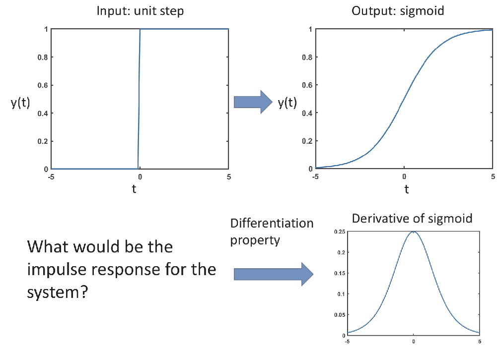
📌 6. Indications of Differentiation

Example:

• Input: Unit step function
• Output: Sigmoid (smooth step-like function)
• Impulse response: Derivative of sigmoid (bell-shaped curve)

  $$h(t) = \frac{d}{dt} \text{sigmoid}(t)$$

✅ The impulse response of a system that turns a unit step into a sigmoid is the derivative of the sigmoid.

System properties for LTI systems

🧠 Memory of an LTI System

• An LTI system is memoryless if:

  $$y(t_0) = \int_{-\infty}^{\infty} x(\tau) h(t_0 - \tau) d\tau$$

  depends only on $x(t_0)$.

• This implies:

  $$h(t_0 - \tau) \neq 0 \text{ only if } \tau = t_0 \Rightarrow h(t) \neq 0 \text{ only if } t = 0$$

• Therefore, the impulse response must be:

  $$h(t) = k\delta(t), \quad \text{for some } k \ne 0$$

• Since convolution with $k\delta(t)$ gives:

  $$x(t) * k\delta(t) = kx(t)$$

  ✅ The only memoryless LTI system is a rescaling system (e.g., amplifier).

⏳ Causality of an LTI System

• General definition: A system is causal if the output $y(t_0)$ depends only on values of the input $x(t)$ for $t \leq t_0$.

• For an LTI system, the output is given by:

  $$y(t_0) = \int_{-\infty}^{\infty} x(\tau) h(t_0 - \tau) d\tau$$

  This must depend only on $x(t)$ for $t \leq t_0$.

• So we must have:

  $$h(t_0 - \tau) = 0 \quad \text{for} \quad \tau > t_0 \Rightarrow h(t) = 0 \quad \text{for} \quad t < 0$$

• ✅ Conclusion: An LTI system is causal iff

  $$h(t) = 0 \quad \text{for } t < 0$$

• This is much easier to check than the general causality definition!

💤 Initial Rest Property

• Definition:
  A system has the initial rest property if the output is zero before the input becomes nonzero.
  In other words:

  The system generates nonzero output only after the input becomes nonzero.

• ⚠️ Note:
  Not all causal or memoryless systems have this property.
  Example: $y(t) = x(t) + 1$ is memoryless and causal, but not initially at rest.

📌 Key Result for LTI Systems:

An LTI system has the initial rest property if and only if it is causal.

---

✍️ Brief Proof:

(1) LTI + Initial Rest ⇒ Causality

• Given: System is LTI and has initial rest ⇒
  For any $x(t)$, if $x(t) = 0$ for $t < t_0$, then $y(t) = 0$ for $t < t_0$.
• Consider the system’s impulse response $h(t)$:
  For the system to output zero before input is nonzero, we must have:

  $$h(t) = 0 \quad \text{for } t < 0$$

  ⇒ By definition, the system is causal.

(2) LTI + Causality ⇒ Initial Rest

• Given: $h(t) = 0$ for $t < 0$ (causality), and system is LTI.
• Let $x(\tau) = 0$ for all $\tau < t_0$. Then for $t < t_0$:

  $$y(t) = \int_{-\infty}^{\infty} x(\tau) h(t - \tau) d\tau = \int_{t_0}^{\infty} x(\tau) h(t - \tau) d\tau$$

  Since $\tau > t_0 > t$, $t - \tau < 0$, and thus $h(t - \tau) = 0$ (by causality),

  $$\Rightarrow y(t) = 0$$

  ⇒ Therefore, the system is initially at rest.

LCCDE Systems

Definition of LCCDE (Linear Constant-Coefficient Differential Equation)

• General form:

  $$\sum_{k=0}^{N} a_k \frac{d^k y(t)}{dt^k} = \sum_{k=0}^{M} b_k \frac{d^k x(t)}{dt^k}$$

  • $y(t)$: output
  • $x(t)$: input

• Order of LCCDE: determined by the highest derivative of $y(t)$, i.e., $N$

• Examples:

  • 0th order: $a_0 y(t) = \sum_{k=0}^M b_k \frac{d^k x(t)}{dt^k}$
  • 1st order: $a_1 \frac{dy(t)}{dt} + a_0 y(t) = \sum_{k=0}^M b_k \frac{d^k x(t)}{dt^k}$
  • 2nd order: $a_2 \frac{d^2 y(t)}{dt^2} + a_1 \frac{dy(t)}{dt} + a_0 y(t) = \sum_{k=0}^M b_k \frac{d^k x(t)}{dt^k}$

• “Constant coefficient”: $a_k$, $b_k$ are constants (not functions of $x, y, t$)

• “Linear”: the equation is a linear combination of derivatives of $y(t)$

⚠️ Note: A system described by an LCCDE is not necessarily a linear system, despite the equation being linear.

Physical Systems Described by LCCDE

Two typical 1st-order LCCDE systems:

---

1. RC Circuit (Example 1.8):
   • Equation:

     $$\frac{dv_c(t)}{dt} + \frac{1}{RC}v_c(t) = \frac{1}{RC}v_s(t)$$

   • Input: $v_s(t)$ (voltage source)
   • Output: $v_c(t)$ (capacitor voltage)
   • Goal: Determine $v_c(t)$'s response to a unit step input.

---

2. Car Motion (Example 1.9):

   • Equation:

     $$\frac{dv(t)}{dt} + \frac{\rho}{m}v(t) = \frac{1}{m}f(t)$$

   • Input: $f(t)$ (applied force)
   • Output: $v(t)$ (car speed)
   • Goal: Determine how speed changes when force is applied suddenly.

---

Both are modeled by first-order LCCDEs and describe dynamic responses to step inputs.

Summary: Solution Space of LCCDE

• To solve an LCCDE:

  $$\sum_{k=0}^{N} a_k \frac{d^k y(t)}{dt^k} = \sum_{k=0}^{M} b_k \frac{d^k x(t)}{dt^k}$$

  we must find all functions $y(t)$ satisfying the equation.

• Solution = Particular Solution 特解 + Homogeneous Solution 通解

  • Particular Solution $y_p(t)$: A specific solution that satisfies the entire non-homogeneous equation.
  • Homogeneous Solution $y_h(t)$: Solution to the homogeneous equation (right-hand side = 0).
    • For example, $y_h(t) = Ae^{-2t}$ for any constant $A$.

• Complete solution space:

  $$y(t) = y_p(t) + y_h(t) = \frac{1}{5}(e^{3t} - e^{-2t})u(t) + Ae^{-2t}$$

• Key fact:
  Every LCCDE has infinitely many solutions, all expressible as:

  $$\text{General solution} = \text{Particular solution} + \text{Homogeneous solution}$$

Initial State

🔹 LCCDE System ≠ LCCDE Equation

• A system built on an LCCDE needs initial state info to produce a unique output.
• Example: A car’s speead response depends not just on the gas pedal (input), but also on its initial speed.

🔹 LCCDE System = LCCDE + Initial State

• Assume input turns on at $t = 0$; $x(t) = 0$ for $t < 0$.
• Initial state: $y(0^-)$ (e.g., initial voltage or velocity).
• Unique solution obtained by matching:

  $$y(0^-) = y_p(0^-) + y_h(A,0^-)$$

Zero-state and Zero-input responses

📌 Definition and Components

• The total output ( y(t) ) of an LCCDE system is:

  $$y(t) = \underbrace{(1 - e^{-t})u(t)}_{\text{Zero-state response}} + \underbrace{y(0^-) e^{-t}}_{\text{Zero-input response}}$$

• Zero-state response:

  • Caused by input signal when initial conditions are zero.
  • Also called the particular solution.

• Zero-input response:

  • Caused by initial conditions when input is zero.
  • Also called the homogeneous solution.

---

🔗 Independence

• The two responses are mutually independent:
  • Changing one does not affect the other.
• Denote:
  • $y_{zi}(t) = y_h(A, t)$, from initial state only.
  • $y_{zs}(t) = y_p(t)$, from input only.
• Therefore:

  $$y(t) = y_{zi}(t) + y_{zs}(t)$$

  is the overall response.

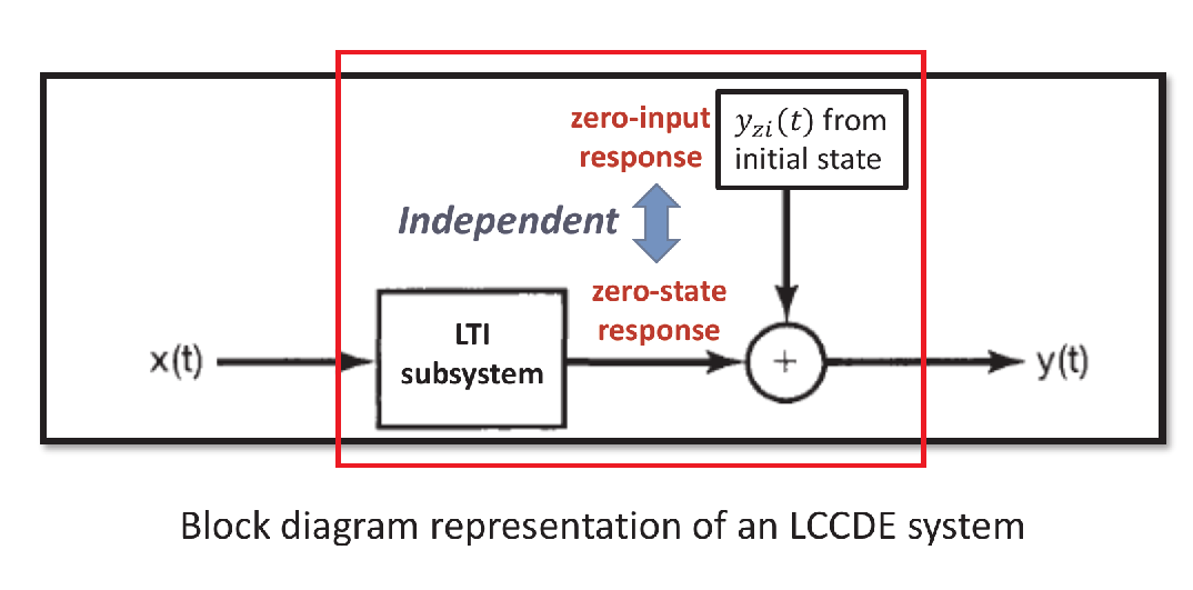
LCCDE is an Incrementally LTI System

• LCCDE output = Zero-state response (LTI) + Zero-input response

  $$y(t) = \mathcal{L}\{x(t)\} + y_{zi}(t)$$

• where

  • $\mathcal{L}\{x(t)\} = y_{zs}(t)$: Response from LTI subsystem, which is also the zero-state reponse

    • This means the zero-state reponse is response from a LTI system

  • $y_{zi}(t)$: Response from initial state, which is also the zero-input response

Key Insight

• A LCCDE is a LTI system if and only if $y_{zi}(t) = 0$ , or more specifically, if and only if the initial state is 0, or the system fits initial rest property.

The “classical approach” to Output prediction for general LCCDE systems

🔸 Motivation

• Predicting output using zero-state and zero-input response can be hard due to the unit-step $u(t)$ in realistic input signals (e.g., $e^{at}u(t), \cos(\omega t)u(t)$).

---

🔸 Classical Approach Strategy

• Remove $u(t)$ and restrict to $t > 0$.

• Solve the modified equation without $u(t)$

  • Let $y(t) = y_p(t) + y_h(A,t)$
  • Guess particular solution $y_p(t)$, Substitute into the equation to determine the coefficients

• adjust using continuity at $t = 0$.

---

🔸 Key Example

1. Problem Setup

• Realistic inputs include unit-step: $x(t) = e^{3t}u(t)$
• Equation:

  $$\frac{dy(t)}{dt} + 2y(t) = e^{3t}u(t), \quad y(0^-) = \gamma$$

---

2. Classical Method Strategy

• Drop $u(t)$ and solve for $t > 0$:

  $$\frac{dy(t)}{dt} + 2y(t) = e^{3t}, \quad t > 0$$

---

3. Solving the Modified Equation

Particular Solution $y_p(t)$:

Guess: $y_p(t) = Ke^{3t}$
Plug into the equation:

$$3Ke^{3t} + 2Ke^{3t} = e^{3t} \Rightarrow 5K = 1 \Rightarrow K = \frac{1}{5}$$

So,

$$y_p(t) = \frac{1}{5}e^{3t}$$

Homogeneous Solution $y_h(t)$:

Solve $\frac{dy_h}{dt} + 2y_h = 0 \Rightarrow y_h(t) = Ae^{-2t}$

---

4. Apply Continuity at $t = 0$

$$y(0^+) = y(0^-) = \gamma$$

$$y(0^+) = \frac{1}{5} + A = \gamma \Rightarrow A = \gamma - \frac{1}{5}$$

---

5. Final Total Solution (for $t > 0$)

$$y(t) = \frac{1}{5}e^{3t} + (\gamma - \frac{1}{5})e^{-2t}$$

---

6. Compare with Original Equation’s Solution

The solution of original equation is

$$y(t) = \frac{1}{5}(e^{3t} - e^{-2t})u(t) + \gamma e^{-2t}u(t)$$

• 有时，题目会给你initial rest条件，然后让你从修改后的方程的解（5的形式）推回原方程完整的解（6的形式），其实一般就是乘上一个 $u(t)$ 就好了

🔸 Interpretation

• Classical and original methods yield the same total output, but decompose it differently:

  • Classical: into forced (particular) and natural (homogeneous) responses
  • Original: into zero-state (particular) and zero-input responses

• However:

  • Particular ≠ zero-state, Homogeneous ≠ zero-input

• To extract components:

  • Zero-Input response: Identify terms $\propto$ (that are directly proportional to) initial state (e.g., $\gamma e^{-2t} \propto \gamma$) → $y_{zi}(t)$
    • It may be a little tricky to extract $y_{zi}(t)$ when the initial state $\gamma$ is a specific number.
    • To tackle this problem, remember that the proportion to initial state is the basic term(s) of the homogenous solution $y_h(t)$ ! (e.g. $e^{-2t}$)
    • Or in another way, the Zero-Input response is also directly proportional to the basic term of homogenous solution $y_h(t)$ (e.g. $\gamma e^{-2t} \propto e^{-2t}$)
  • Zero-State response: Remaining terms → $y_{zs}(t)$

---

🔸 Summary Table (Common Particular Solution for input)

Input $x(t)$	Modified Input	Particular Solution
$E u(t)$	$E$ (Constant)	$K$
$t^p u(t)$	$t^p$	$\sum_{i=0}^{p} K_i t^{i}$
$e^{at} u(t)$	$e^{at}$	$K e^{at}$
$\cos(\omega t) u(t)$	$\cos(\omega t)$	$K_1\cos(\omega t) + K_2\sin(\omega t)$

---

🔸 Notes

• Classical approach gives correct output but lacks clear separation of zero-state/zero-input.
• Better tools (e.g., Laplace Transform) will be introduced for direct prediction.

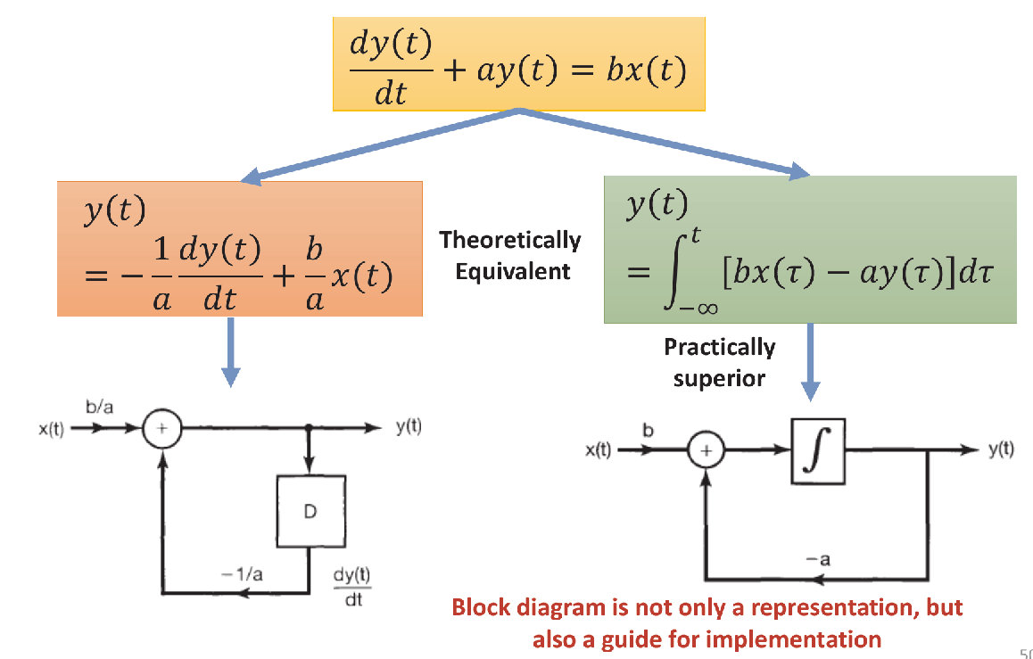
Block diagram representations of LCCDE systems

There are 3 common modules: differentiator, multiplication, and addition. They are represented by:

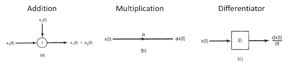
And the intergrator is represented by

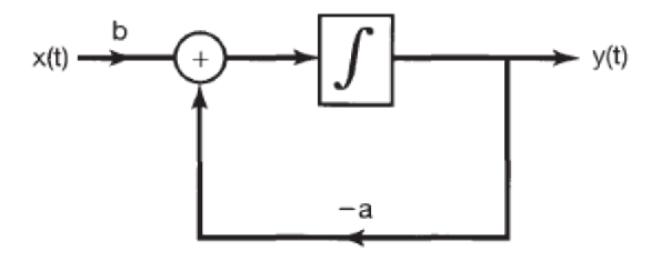
Multiple forms

There can be multiple block diagrams to represent the same system, based on different reformulation of the LCCDE.

• For example, you can use a differentiator instead of an integrator
• Although the two forms are theoretically equivalent, implementation using integrator is better that that using differentiator due to improved robustness of integrator against noise.