Chapter4 Continuous-time Fourier Transform

IV. From Fourier Series to Fourier Transform 🌉

A. Motivation

Fourier series is powerful for periodic signals, but most real-world signals are non-periodic. We need a way to analyze these non-periodic signals in the frequency domain.

B. The Basic Idea

A non-periodic signal can be viewed as a periodic signal with an infinite period ($T \rightarrow \infty$).

• As $T$ increases for a sequence of periodic signals (each replicating a finite-duration aperiodic signal $x(t)$ within its period), the periodic signals converge to the non-periodic signal $x(t)$.
• Correspondingly, their spectra (which are line spectra) should converge to the spectrum of the non-periodic signal. As $T \rightarrow \infty$, the fundamental frequency $\omega_0 = 2\pi/T \rightarrow 0$, meaning the lines in the spectrum become infinitely close, forming a continuous spectrum.

C. Deriving the Fourier Transform

Step 1: Construct a periodic signal $\tilde{x}_T(t)$

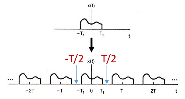
• Let $x(t)$ be a non-periodic signal such that $x(t)=0$ for $|t|>T_1$.
• Construct a periodic signal $\tilde{x}_T(t)$ with period $T > 2T_1$, such that $\tilde{x}_T(t) = x(t)$ for $|t| < T/2$.
• Then, $\lim_{T\rightarrow\infty}\tilde{x}_{T}(t)=x(t)$.
• Since $\tilde{x}_T(t)$ is periodic (with $\omega_0 = 2\pi/T$), its Fourier series coefficients are:

  $$a_k = \frac{1}{T}\int_{-T/2}^{T/2}\tilde{x}_{T}(t)e^{-jk\omega_{0}t}dt$$

• And the series is $\tilde{x}_{T}(t)=\sum_{k=-\infty}^{\infty}a_{k}e^{jk\omega_{0}t}$.

Step 2: Derive the Fourier Transform Analysis Equation

• From the coefficient formula:

  $$Ta_k = \int_{-T/2}^{T/2}\tilde{x}_{T}(t)e^{-jk\omega_{0}t}dt$$

• Since $\tilde{x}_T(t) = x(t)$ in the interval $[-T/2, T/2]$ when $T \to \infty$, we have the following conclusion when $T \to \infty$ :

  $$Ta_k = \int_{-\frac{T}{2}}^{\frac{T}{2}}x(t)e^{-jk\omega_{0}t}dt = \int_{-\infty}^{\infty}x(t)e^{-jk\omega_{0}t}dt$$

• Let’s define $X(j\omega) \triangleq \int_{-\infty}^{\infty}x(t)e^{-j\omega t}dt$ as the Fourier Transform of $x(t)$.

• Then, $Ta_k = X(j\omega)|_{\omega=k\omega_0}$.

• The quantity $Ta_k$ represents samples of the envelope $X(j\omega)$. As $T \rightarrow \infty$, $\omega_0 \rightarrow 0$, and the discrete samples $k\omega_0$ become a continuous variable $\omega$.

• Thus, as $T \rightarrow \infty$, $Ta_k \rightarrow X(j\omega)$, which is the spectrum of the non-periodic signal $x(t)$.

• The analysis equation of Fourier Transform is:

$$X(j\omega)=\int_{-\infty}^{\infty}x(t)e^{-j\omega t}dt$$

Step 3: Derive the Fourier Transform Synthesis Equation

• Start with the Fourier series for $\tilde{x}_T(t)$:

  $$\tilde{x}_{T}(t)=\sum_{k=-\infty}^{\infty}a_{k}e^{jk\omega_{0}t}$$

• Substitute $a_k = \frac{1}{T}X(jk\omega_0)$:

  $$\tilde{x}_{T}(t)=\sum_{k=-\infty}^{\infty}\frac{1}{T}X(jk\omega_{0})e^{jk\omega_{0}t}$$

• Since $\omega_0 = 2\pi/T$, we have $1/T = \omega_0/(2\pi)$:

  $$\tilde{x}_{T}(t) = \frac{1}{2\pi}\sum_{k=-\infty}^{\infty}X(jk\omega_{0})e^{jk\omega_{0}t}\omega_{0}$$

• This sum can be seen as an approximation of an integral. Each term $X(jk\omega_{0})e^{jk\omega_{0}t}\omega_{0}$ represents the area of a rectangle of height $X(jk\omega_{0})e^{jk\omega_{0}t}$ and width $\omega_0$.

  • Actually this fits the definition method of Riemann Integral.

• As $T \rightarrow \infty$, $\omega_0 \rightarrow 0$, and $\tilde{x}_T(t) \rightarrow x(t)$. The sum becomes an integral:

  $$x(t) = \lim_{\omega_0 \rightarrow 0} \frac{1}{2\pi}\sum_{k=-\infty}^{\infty}X(jk\omega_{0})e^{jk\omega_{0}t}\omega_{0} = \frac{1}{2\pi}\int_{-\infty}^{\infty}X(j\omega)e^{j\omega t}d\omega$$

  This is the synthesis equation (Inverse Fourier Transform).

Summary of Derivation:

1. Given a non-periodic $x(t)$ (compactly supported, though this can be relaxed in formal proof), construct periodic $\tilde{x}_T(t)$ such that $\lim_{T\rightarrow\infty}\tilde{x}_{T}(t)=x(t)$.
2. Show that as $T\rightarrow\infty$, $Ta_k \rightarrow X(j\omega) \triangleq \int_{-\infty}^{\infty}x(t)e^{-j\omega t}dt$. Define $X(j\omega)$ as the spectrum of $x(t)$.
3. Show that as $T\rightarrow\infty$, $\sum a_k e^{jk\omega_0 t}$ converges to $\frac{1}{2\pi}\int X(j\omega)e^{j\omega t}d\omega$. Thus, $x(t) = \frac{1}{2\pi}\int X(j\omega)e^{j\omega t}d\omega$ is the synthesis equation.

---

V. Fourier and Inverse Fourier Transforms 🔄

The Fourier Transform pair is defined as:

• Fourier Transform (Analysis Equation):

  $$X(j\omega) = \mathfrak{F}\{x(t)\} = \int_{-\infty}^{\infty}x(t)e^{-j\omega t}dt$$

  • This transforms the signal $x(t)$ into its spectrum $X(j\omega)$.

• Inverse Fourier Transform (Synthesis Equation):

  $$x(t) = \mathfrak{F}^{-1}\{X(j\omega)\} = \frac{1}{2\pi}\int_{-\infty}^{\infty}X(j\omega)e^{j\omega t}d\omega$$

  • This synthesizes the signal $x(t)$ from its spectrum $X(j\omega)$.

• There is a notable symmetry between the transform and its inverse.

Comparison with Fourier Series:

Synthesis Equations:

• Periodic: $x_{T_{0}}(t)=\sum_{k=-\infty}^{+\infty}a_{k}e^{jk\omega_{0}t}$ (linear combination of harmonically related complex exponentials (HRCEs) with fundamental frequency $\omega_0$).
• Non-periodic: $x(t)=\frac{1}{2\pi}\int_{-\infty}^{\infty}X(j\omega)e^{j\omega t}d\omega$ (linear combination of HRCEs with an infinitely small fundamental frequency).

Analysis Equations:

• Periodic: $a_{k}=\frac{1}{T_{0}}\int_{T_{0}}x_{T_{0}}(t)e^{-jk\omega_{0}t}dt$ (generates a discrete spectrum).
• Non-periodic: $X(j\omega)=\int_{-\infty}^{\infty}x(t)e^{-j\omega t}dt$ (generates a continuous spectrum as “effective fundamental frequency” is $d\omega \rightarrow 0$).

---

VI. Examples of Fourier Transforms 🧮

Example 1: $x(t)=e^{-at}u(t)$, for $a>0$

$$\begin{align} X(j\omega) &= \int_{-\infty}^{\infty}e^{-at}u(t)e^{-j\omega t}dt = \int_{0}^{\infty}e^{-(a+j\omega)t}dt \\ &= \left[\frac{e^{-(a+j\omega)t}}{-(a+j\omega)}\right]_{0}^{\infty} = 0 - \frac{1}{-(a+j\omega)} = \frac{1}{a+j\omega} \end{align}$$

• Magnitude: $|X(j\omega)| = \frac{1}{\sqrt{a^2+\omega^2}}$.
• Phase: $\angle X(j\omega) = -\text{atan}(\frac{\omega}{a})$.
• Note: $X(j0) = \int_{-\infty}^{\infty}x(t)dt = 1/a$.

Example 2: $x(t)=e^{-a|t|}$, for $a>0$
$X(j\omega) = \int_{-\infty}^{0}e^{at}e^{-j\omega t}dt + \int_{0}^{\infty}e^{-at}e^{-j\omega t}dt$
$X(j\omega) = \int_{0}^{\infty}e^{-at}e^{j\omega t}dt + \int_{0}^{\infty}e^{-at}e^{-j\omega t}dt$ (by changing variable $t \rightarrow -t$ in the first integral)
$X(j\omega) = \int_{0}^{\infty}e^{-(a-j\omega)t}dt + \int_{0}^{\infty}e^{-(a+j\omega)t}dt$
$X(j\omega) = \frac{1}{a-j\omega} + \frac{1}{a+j\omega} = \frac{(a+j\omega) + (a-j\omega)}{(a-j\omega)(a+j\omega)} = \frac{2a}{a^2+\omega^2}$.

• Magnitude: $|X(j\omega)| = X(j\omega)$ (since it’s real and positive).
• Phase: $\angle X(j\omega) = 0$.

Example 3: $x(t)=\delta(t)$ (Dirac delta function)
$X(j\omega) = \int_{-\infty}^{\infty}\delta(t)e^{-j\omega t}dt = e^{-j\omega \cdot 0} = 1$ (by the sifting property of the delta function).
The spectrum is constant, meaning $\delta(t)$ is composed of all frequencies with equal strength (amplitude 1 and phase 0).

---

VII. Convergence of the Fourier Transform 📈

The convergence criteria for Fourier Transform are inherited from those for Fourier Series, as FT is effectively FS when $T \rightarrow \infty$.

Two types of convergence:

1. Finite Energy Condition: If $x(t)$ has finite energy, i.e., $\int_{-\infty}^{\infty}|x(t)|^{2}dt<\infty$, then the Fourier Transform converges in the sense that the error $\int_{-\infty}^{\infty}|x(t)-\hat{x}(t)|^{2}dt=0$, where $\hat{x}(t) = \mathfrak{F}^{-1}\{\mathfrak{F}\{x(t)\}\}$. Such signals are often bounded and decay to 0 sufficiently fast as $|t|\rightarrow\infty$.
2. Dirichlet Conditions: If $x(t)$ satisfies the Dirichlet conditions, $\hat{x}(t)$ converges pointwise to $x(t)$ where $x(t)$ is continuous, and to the average of the values on either side of a discontinuity.
   The Dirichlet conditions are:
   a. $x(t)$ is absolutely integrable over the entire time domain: $\int_{-\infty}^{\infty}|x(t)|dt < \infty$. 绝对可积
   b. $x(t)$ has a finite number of maxima and minima within any finite interval. 有限个极值点
   c. $x(t)$ has a finite number of discontinuities, each with a finite height, within any finite interval. 有限个间断点，且都是第一类间断点

• For $x(t)=e^{-at}u(t), a>0$: Satisfies Dirichlet conditions.
• For $x(t)=e^{-a|t|}, a>0$: Satisfies Dirichlet conditions.
• For $x(t)=\delta(t)$: Violates the third Dirichlet condition (infinite discontinuity). However, its FT is still considered to converge because Dirichlet conditions are sufficient, not necessary.

---

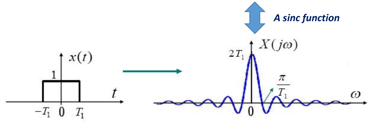
VIII. Rectangle-Sinc Fourier Transform Pair

If $X(j\omega) = \mathcal{F}\{x(t)\}$, then $x(t)$ and $X(j\omega)$ are a Fourier transform pair. The rectangle-sinc pair is very important.

Example 4.4: Rectangular Pulse in Time Domain

Let $x(t) = \begin{cases} 1, & |t|<T_1 \\ 0, & |t|>T_1 \end{cases}$.

$$\begin{align} X(j\omega) &= \int_{-T_1}^{T_1} 1 \cdot e^{-j\omega t}dt = \left[\frac{e^{-j\omega t}}{-j\omega}\right]_{-T_1}^{T_1} \\ \implies X(j\omega) &= \frac{e^{-j\omega T_1} - e^{j\omega T_1}}{-j\omega} = \frac{-(e^{j\omega T_1} - e^{-j\omega T_1})}{-j\omega} = \frac{2j\sin(\omega T_1)}{j\omega} = \frac{2\sin(\omega T_1)}{\omega} \end{align}$$

• This is a sinc-like function.
• At $\omega=0$: Using L’Hopital’s Rule, $\lim_{\omega\to 0} \frac{2\sin(\omega T_1)}{\omega} = \lim_{\omega\to 0} \frac{2T_1\cos(\omega T_1)}{1} = 2T_1$.
• Zero crossings: $\frac{2\sin(\omega T_1)}{\omega} = 0$ when $\sin(\omega T_1)=0$ and $\omega \neq 0$. So, $\omega T_1 = k\pi$ for $k \in \mathbb{Z}, k \neq 0$, i.e., $\omega = k\pi/T_1$.
• It’s an even symmetric function.

Normalized Sinc Function:
The normalized sinc function is defined as:

$$\text{sinc}(x) = \frac{\sin(\pi x)}{\pi x}$$

• $\text{sinc}(0)=1$.
• Zero crossings at all non-zero integers $k$ (i.e., $x=k, k \neq 0$)

Using this, the Fourier transform of the rectangular pulse $x(t)$ can be written as:

$$\frac{2\sin(\omega T_1)}{\omega} = 2T_1 \frac{\sin(\omega T_1)}{\omega T_1} = 2T_1 \frac{\sin(\pi \cdot \frac{\omega T_1}{\pi})}{\pi \cdot \frac{\omega T_1}{\pi}} = 2T_1 \text{sinc}\left(\frac{\omega T_1}{\pi}\right) \text{ or } 2T_1 \text{sinc}\left(\frac{T_1}{\pi}\omega\right)$$

Example 4.5: Rectangular Pulse in Frequency Domain (Ideal Lowpass Filter Spectrum)
Let $X(j\omega) = \begin{cases} 1, & |\omega|<W \\ 0, & |\omega|>W \end{cases}$
We use the inverse Fourier transform to find $x(t)$:

$$\begin{align} x(t) &= \frac{1}{2\pi}\int_{-W}^{W} 1 \cdot e^{j\omega t}d\omega = \frac{1}{2\pi}\left[\frac{e^{j\omega t}}{jt}\right]_{-W}^{W} \\ \implies x(t) &= \frac{1}{2\pi} \frac{e^{jWt} - e^{-jWt}}{jt} = \frac{1}{2\pi} \frac{2j\sin(Wt)}{jt} = \frac{\sin(Wt)}{\pi t} \end{align}$$

This can also be written using the normalized sinc function:

$$\frac{\sin(Wt)}{\pi t} = \frac{W}{\pi} \frac{\sin(Wt)}{Wt} = \frac{W}{\pi} \text{sinc}\left(\frac{Wt}{\pi}\right)$$

---

IX. Duality of Fourier Transform ✨

There’s an interesting observation:

• A rectangular signal in time, $x(t)$, has a sinc-shaped spectrum, $X(j\omega)$.
• A rectangular spectrum in frequency, $X(j\omega)$, corresponds to a sinc-shaped signal in time, $x(t)$.

Duality Property: If a signal $x(t)$ has a spectrum $X(j\omega)$ (i.e., $x(t) \leftrightarrow X(j\omega)$), then a signal in time that has the functional form of $X(t)$ will have a spectrum $2\pi x(-\omega)$ (i.e., $X(t) \leftrightarrow 2\pi x(-\omega)$). This will be formally proven in the next lecture.

Lecture 9: Fourier Transform Properties

FT and FS (Fourier Series)

The Fourier Series (FS) represents a periodic signal $\chi_{T_{0}}(t)$ as a sum of weighted harmonics, while the Fourier Transform (FT) represents a signal $x(t)$ in the continuous frequency domain.

• Fourier Series:

  $$\begin{cases} a_{k}=\frac{1}{T_{0}}\int_{T_{0}}\chi_{T_{0}}(t)e^{-jk\omega_{0}t}dt \\ \chi_{T_{0}}(t)=\sum_{k=-\infty}^{+\infty}a_{k}e^{jk\omega_{0}t} \end{cases}$$

• Fourier Transform:

  $$\begin{cases} X(j\omega)=\int_{-\infty}^{\infty}x(t)e^{-j\omega t}dt \\ x(t)=\frac{1}{2\pi}\int_{-\infty}^{\infty}X(j\omega)e^{j\omega t}d\omega \end{cases}$$

Key Differences:

• The Fourier series spectrum ($a_k$) is a discrete-time signal, leading to a sum in the synthesis equation.
• The Fourier transform spectrum ($X(j\omega)$) is a continuous-time signal, leading to an integral in the synthesis equation.
• These differences arise because a non-periodic signal can be seen as having an infinite period, so its representation includes harmonics at all frequencies.

---

Normalized sinc Function

The normalized sinc function is defined as:

$$sinc(\omega)=\frac{sin(\pi\omega)}{\pi\omega}$$

An arbitrary rectangular pulse $x(t)$ which is 1 for $|t| < T_1$ and 0 otherwise, has a Fourier Transform:

$$X(j\omega) = \frac{2\sin(\omega T_{1})}{\omega}$$

This can be rewritten using the normalized sinc function:

$$X(j\omega) = 2T_{1}sinc(\frac{T_{1}}{\pi}\omega)$$

---

Fourier Transform for Periodic Signals

To find the FT spectrum of a periodic signal $x_{T_{0}}(t)$, we look for $X(j\omega)$ such that:

$$x_{T_{0}}(t)=\frac{1}{2\pi}\int_{-\infty}^{\infty}X(j\omega)e^{j\omega t}d\omega$$

If $a_k$ are the FS coefficients of $x_{T_{0}}(t)$, then we must have:

$$\frac{1}{2\pi}\int_{-\infty}^{\infty}X(j\omega)e^{j\omega t}d\omega=\sum_{k=-\infty}^{\infty}a_{k}e^{jk\omega_{0}t}$$

This implies that $X(j\omega)$ must be an impulse train located at the harmonic frequencies $k\omega_{0}$.

So, the Fourier Transform of a periodic signal $x_{T_{0}}(t)$ with Fourier Series coefficients $a_k$ is (a weighted impulse train):

$$X(j\omega) \triangleq 2\pi\sum_{k=-\infty}^{\infty}a_{k}\delta(\omega-k\omega_{0})$$

Verification:
Substituting this $X(j\omega)$ into the inverse FT equation:

$$\begin{align} x_{T_{0}}(t) &= \frac{1}{2\pi}\int_{-\infty}^{\infty} (2\pi\sum_{k=-\infty}^{\infty}a_{k}\delta(\omega-k\omega_{0})) e^{j\omega t}d\omega \\ x_{T_{0}}(t) &= \sum_{k=-\infty}^{\infty}a_{k}\int_{-\infty}^{\infty}\delta(\omega-k\omega_{0})e^{j\omega t}d\omega = \sum_{k=-\infty}^{\infty}a_{k}e^{jk\omega_{0}t} \end{align}$$

This is the Fourier series synthesis equation, confirming the result.

Convergence Note: Periodic signals don’t satisfy the Dirichlet conditions or finite energy criterion for FT convergence. However, convergence is still guaranteed here because these conditions are sufficient, not necessary.

---

Examples of FT for Periodic Signals

1. $x(t) = cos(\omega_{0}t)$

   • FS coefficients: $a_1 = 1/2$, $a_{-1} = 1/2$, and $a_k = 0$ for other $k$.
   • FT: $X(j\omega) = \pi\delta(\omega-\omega_{0}) + \pi\delta(\omega+\omega_{0})$
   • Difference between FT and FS spectra: The FT spectrum consists of impulses (not just numbers), is rescaled by $2\pi$, and the horizontal axis represents $\omega$ instead of $k$.

2. $x(t) = \sin (\omega_0 T)$

   • FS coefficients: $a_1 = \frac{1}{2j}$, $a_{-1} = -\frac{1}{2j}$, and $a_k = 0$ for other $k$.
   • FT: $X(j\omega) = \frac{\pi}{j}[\delta(\omega - \omega_0) - \delta(\omega + \omega_0)] = j\pi[\delta(\omega + \omega_0) - \delta(\omega - \omega_0)]$

3. $x(t) = \sum_{n=-\infty}^{\infty}\delta(t-nT)$ (Comb function / Periodic impulse train)

   • FS coefficients: $a_k = \frac{1}{T}$ for all $k$.
   • FT: $X(j\omega) = \frac{2\pi}{T}\sum_{k=-\infty}^{\infty}\delta(\omega-\frac{2\pi}{T}k)$
   • The Fourier transform of a comb function is another comb function with an inversely proportional period.

4. Periodic Square Signal $\tilde{x}(t)$ (1 for $|t|<T_1$, 0 for $T_1<|t|\leq T_0/2$, period $T_0$)

   • FS coefficients: $a_{k}=\frac{sin(\frac{2\pi}{T_{0}}kT_{1})}{\pi k}$
   • FT: $X(j\omega)=\sum_{k=-\infty}^{\infty}\frac{2\sin(\frac{2\pi}{T_{0}}kT_{1})}{k}\delta(\omega-\frac{2\pi}{T_{0}}k)$
     • This can also be written as: $X(j\omega) = \frac{4\pi T_{1}}{T_{0}}sinc(\frac{T_{1}}{\pi}\omega)\sum_{k=-\infty}^{\infty}\delta(\omega-\frac{2\pi}{T_{0}}k)$
   • The FT spectrum of a periodic square wave is a sampled sinc function.

A table of basic Fourier Transform pairs is provided, and it’s highly recommended to memorize them.

Question Example: Evaluate and plot the FT spectrum of $1+cos(\omega_{0}t)+sin(2\omega_{0}t)$.

$$1+cos(\omega_{0}t)+sin(2\omega_{0}t) = 1+\frac{1}{2}e^{j\omega_{0}t}+\frac{1}{2}e^{-j\omega_{0}t}+\frac{1}{2j}e^{j2\omega_{0}t}-\frac{1}{2j}e^{-j2\omega_{0}t}$$

FS coefficients $a_k$:
$a_0 = 1$
$a_1 = 1/2$, $a_{-1} = 1/2$
$a_2 = 1/(2j)$, $a_{-2} = -1/(2j)$
FT Spectrum: $X(j\omega) = 2\pi\sum a_k \delta(\omega - k\omega_0)$

$$X(j\omega) = 2\pi\delta(\omega) + \pi\delta(\omega-\omega_0) + \pi\delta(\omega+\omega_0) + \frac{\pi}{j}\delta(\omega-2\omega_0) - \frac{\pi}{j}\delta(\omega+2\omega_0)$$

---

Properties of Fourier Transform

1. Linearity

   • If $x(t)\leftrightarrow X(j\omega)$ and $y(t)\leftrightarrow Y(j\omega)$, then $ax(t)+by(t)\leftrightarrow aX(j\omega)+bY(j\omega)$ for any complex numbers $a$ and $b$.
   • This is true because integration is a linear operation.

2. Time-Shifting Property: If $x(t)\leftrightarrow X(j\omega)$, then $x(t-t_{0})\leftrightarrow e^{-j\omega t_{0}}X(j\omega)$

   • For FS: $x(t-t_{0})\stackrel{F.S.}{\longleftrightarrow} e^{-jk\omega_{0}t_{0}}a_{k}$
   • Indication: Time shifting only changes the phase spectrum by adding a linear phase $-\omega t_{0}$. The phase spectrum determines the location of each harmonic.

3. Time-Reversal: If $x(t)\leftrightarrow X(j\omega)$, then $x(-t)\leftrightarrow X(-j\omega)$

   • For FS: $x(-t)\leftrightarrow a_{-k}$
   • Indications:
     • If $x(t)$ is even, then $X(j\omega)$ is even.
     • If $x(t)$ is odd, then $X(j\omega)$ is odd.
   • Reversing a signal or flipping an image causes a reversed or flipped spectrum.

4. Conjugacy and Symmetry
   If $x(t)\leftrightarrow X(j\omega)$, then $x^{*}(t)\leftrightarrow X^{*}(-j\omega)$

   • For FS: $x^{*}(t)\leftrightarrow a_{-k}^{*}$

   • If $x(t)$ is real, then $X(j\omega)=X^{*}(-j\omega)$ (conjugate symmetric).

     • This means the real part of $X(j\omega)$ is even, and the imaginary part of $X(j\omega)$ is odd.

   • For real signals $x(t)$:

     • If $x(t)$ is real and even, $X(j\omega)$ is real and even.
     • If $x(t)$ is real and odd, $X(j\omega)$ is imaginary and odd.

   • Since a real signal $x(t) = x_e(t) + x_o(t)$ (even and odd components), its FT is $X(j\omega) = \mathcal{F}\{x_e(t)\} + \mathcal{F}\{x_o(t)\}$.

   • Also, $X(j\omega) = Re\{X(j\omega)\} + j \cdot Im\{X(j\omega)\}$.

   • This implies: $Re\{X(j\omega)\} = \mathcal{F}\{x_e(t)\}$ and $jIm\{X(j\omega)\} = \mathcal{F}\{x_o(t)\}$.

   Example 4.9 (Combining signals):

   How to generate Fourier transform of x(t) from that of x1(t) & x2(t)?

   
   • Given $x_1(t)$ with $X_1(j\omega) = \frac{2\sin(\omega/2)}{\omega}$ and $x_2(t)$ with $X_2(j\omega) = \frac{2\sin(3\omega/2)}{\omega}$.
   • Find that $x(t) = \frac{1}{2}x_1(t-2.5) + x_2(t-2.5)$.
   • Then $X(j\omega) = e^{-j2.5\omega} \left( \frac{1}{2}X_1(j\omega) + X_2(j\omega) \right) = e^{-j2.5\omega} \left( \frac{\sin(\omega/2)}{\omega} + \frac{2\sin(3\omega/2)}{\omega} \right)$.

   Example 4.10 (Using properties to find FT): Find FT of $x(t) = e^{-a|t|}$, $a>0$, given $e^{-at}u(t) \leftrightarrow \frac{1}{a+j\omega}$.

   • Decompose $x(t)$ into $x(t) = e^{-at}u(t) + e^{at}u(-t)$.
   • Let $y(t) = e^{-at}u(t)$. Then $e^{at}u(-t) = y(-t)$
   • Then, we have $Y(j\omega) = \frac{1}{a+j\omega}$, and $\mathcal{F}\{y(-t)\} = Y(-j\omega) = \frac{1}{a-j\omega}$.
   • So, $X(j\omega) = \frac{1}{a+j\omega} + \frac{1}{a-j\omega} = \frac{a-j\omega + a+j\omega}{(a+j\omega)(a-j\omega)} = \frac{2a}{a^2+\omega^2}$.
   • Alternatively, $x(t) = 2 \cdot \text{Ev}\{e^{-at}u(t)\}$.
   • Since $\text{Ev}\{y(t)\} \leftrightarrow Re\{Y(j\omega)\}$,
   • $X(j\omega) = 2 \cdot Re\left\{\frac{1}{a+j\omega}\right\} = 2 \cdot Re\left\{\frac{a-j\omega}{a^2+\omega^2}\right\} = 2 \cdot \frac{a}{a^2+\omega^2} = \frac{2a}{a^2+\omega^2}$.

5. Multiplication Property

   $$x(t)y(t) \stackrel{\mathcal{F}}{\leftrightarrow} \frac{1}{2\pi} X(j\omega) * Y(j\omega)$$

6. Differentiation & Integration

   • Differentiation Property: If $x(t)\leftrightarrow X(j\omega)$, then $\frac{dx(t)}{dt}\leftrightarrow j\omega X(j\omega)$
     • For FS: $\frac{dx(t)}{dt}\stackrel{F.S.}{\longleftrightarrow} jk\omega_{0}a_{k}$
     • Indication: A differentiator acts as a highpass filter (non-ideal).
   • Integration Property: If $x(t)\leftrightarrow X(j\omega)$, then $\int_{-\infty}^{t}x(\tau)d\tau\leftrightarrow\frac{1}{j\omega}X(j\omega) + \pi X(j0)\delta(\omega)$
     • The term $\pi X(j0)\delta(\omega)$ accounts for the DC component or average value that can result from integration.
     • For FS: If $a_0=0$, then $\int_{-\infty}^{t}x(\tau)d\tau \stackrel{F.S.}{\longleftrightarrow} \frac{a_k}{jk\omega_0}$ (assuming $x(t)$ is the signal being integrated, not $\tau$).

   Example 4.11 (FT of unit step): Find FT for $x(t)=u(t)$.

   • We know $u(t) = \int_{-\infty}^{t}\delta(\tau)d\tau$. Let $g(t) = \delta(t)$, so $G(j\omega)=1$.
     Using the integration property:

     $$X(j\omega) = \frac{G(j\omega)}{j\omega} + \pi G(j0)\delta(\omega) = \frac{1}{j\omega} + \pi(1)\delta(\omega) = \frac{1}{j\omega} + \pi\delta(\omega)$$

     We can recover the FT of $\delta(t)$ using differentiation:

     $$\delta(t) = \frac{du(t)}{dt} \leftrightarrow j\omega \left( \frac{1}{j\omega} + \pi\delta(\omega) \right) = 1 + j\omega\pi\delta(\omega)$$

     Since $\omega\delta(\omega) = 0$, this simplifies to $1$.

7. Parseval’s Theorem
   If $x(t)\leftrightarrow X(j\omega)$, then $\int_{-\infty}^{\infty}|x(t)|^{2}dt=\frac{1}{2\pi}\int_{-\infty}^{\infty}|X(j\omega)|^{2}d\omega$

   • This is also called the “energy-preservation property”.
   • $|X(j\omega)|^2$ is called the Energy-density Spectrum（功率密度谱，简称功率谱） of $x(t)$, reflecting energy density at each frequency.
   • For natural signals, energy is typically more concentrated in lower frequencies.

8. Time-Scaling Property
   If $x(t)\stackrel{\mathcal{F}}{\leftrightarrow} X(j\omega)$, then for any real $a \neq 0$: $x(at)\stackrel{\mathcal{F}}{\leftrightarrow} \frac{1}{|a|}X(\frac{j\omega}{a})$

   • If $|a|>1$, $x(t)$ is squeezed, $X(j\omega)$ is stretched and scaled down.
   • If $|a|<1$, $x(t)$ is stretched, $X(j\omega)$ is squeezed and scaled up.
   • Squeezing in time (faster variation) leads to more high-frequency components (stretching in frequency).
   • Stretching in time (slower variation) leads to more low-frequency components (squeezing in frequency).
   • Example: $rect(t/T_1) \leftrightarrow 2|T_1|sinc(\frac{T_1\omega}{\pi})$, where $rect(t)=1$ for $|t|<1$ and 0 otherwise. (Note: The slide shows $rect(t)\leftrightarrow2sinc(\frac{\omega}{\pi})$ with $T_1=1$ for the basic form).

   Proof of Time-Scaling Property:
   $\mathcal{F}\{x(at)\} = \int_{-\infty}^{\infty} x(at)e^{-j\omega t}dt$.
   Let $u = at$, so $t = u/a$ and $dt = du/a$.
   If $a > 0$:
   $\int_{-\infty}^{\infty} x(u)e^{-j\omega (u/a)} \frac{du}{a} = \frac{1}{a} \int_{-\infty}^{\infty} x(u)e^{-j(\omega/a)u}du = \frac{1}{a}X(j\frac{\omega}{a})$.
   If $a < 0$: The limits of integration flip, $\int_{\infty}^{-\infty}$, which introduces a negative sign that cancels with $1/a$ when taking $|a|$.
   $\int_{\infty}^{-\infty} x(u)e^{-j\omega (u/a)} \frac{du}{a} = -\frac{1}{a} \int_{-\infty}^{\infty} x(u)e^{-j(\omega/a)u}du = \frac{1}{|a|}X(j\frac{\omega}{a})$.
   Thus, for $a \neq 0$, $\mathcal{F}\{x(at)\} = \frac{1}{|a|}X(j\frac{\omega}{a})$.

9. Duality and Related Properties
   The FT and IFT equations are symmetric, differing mainly by a sign in the exponent and a $1/(2\pi)$ scaler.

   $$X(j\omega)=\int_{-\infty}^{\infty}x(t)e^{-j\omega t}dt \quad x(t)=\frac{1}{2\pi}\int_{-\infty}^{\infty}X(j\omega)e^{j\omega t}d\omega$$

   Duality Property:
   If $x(t)\leftrightarrow X(j\omega)$, then $X(t)\leftrightarrow 2\pi x(-j\omega)$ , or equivalently, $\frac{1}{2\pi}X(-t)\leftrightarrow x(j\omega)$

   Proof of $\frac{1}{2\pi}X(-t)\leftrightarrow x(j\omega)$:

   The provided proof in the slide is for $\mathcal{F}^{-1}\{x(j\omega)\} = \frac{1}{2\pi}X(-t)$:

   $$\mathcal{F}^{-1}\{x(j\omega)\} = \frac{1}{2\pi}\int_{-\infty}^{\infty} x(j\omega)e^{j\omega t} d\omega = \frac{1}{2\pi}\int_{-\infty}^{\infty} x(j\omega)e^{-j\omega(-t)} d\omega = \frac{1}{2\pi}X(-t)$$

   Alternative Proof
   Consider the original IFT

   $$x(t) = \frac{1}{2\pi}\int_{-\infty}^{\infty}X(j\omega)e^{j\omega t}d\omega$$

   Swap variables $\omega \leftrightarrow t$ , we have

   $$x(j\omega) = \frac{1}{2\pi}\int_{-\infty}^{\infty}X(t)e^{jt\omega}dt = \frac{1}{2\pi} \int_{\infty}^{-\infty}X(-t)e^{j(-t)\omega}d(-t) = \frac{1}{2\pi} \int_{-\infty}^{\infty} X(-t)e^{-j\omega t}\, dt$$

   This expression is $x(j\omega) = \mathcal{\frac{1}{2\pi} F}\{X(-t)\}$

   Applications of Duality - Deriving New Properties:

   • Frequency-Shifting Property:

   $$x(t)e^{j\omega_{0}t}\leftrightarrow X(j(\omega-\omega_{0}))$$

   Derived from time-shifting property and duality.
   Proof:

   • Time-shifting: $x(t-t_0) \leftrightarrow e^{-j\omega t_0}X(j\omega)$.
   • Let $x(t) \stackrel{\mathcal{F}}{\leftrightarrow} X(j\omega)$
   • Duality: $X(t) \leftrightarrow 2\pi x(-j\omega)$.
   • Apply time shift to $X(t)$: $X(t-\omega_0) \leftrightarrow 2\pi x(-j\omega)e^{-j\omega\omega_0}$.
   • Use Duality Again: $\frac{1}{2\pi} Y(-t) \leftrightarrow y(j\omega)$ where $y(t) = X(t-\omega_0)$ and $Y(j\omega) = 2\pi x(-j\omega) e^{-j\omega \omega_0}$
   • Finally, we have

$$\frac{1}{2\pi} \cdot 2\pi \cdot x(t) e^{-jt\omega_0} \stackrel{\mathcal{F}}{\leftrightarrow} X(j(\omega-\omega_0)) \implies x(t) e^{-jt\omega_0} \stackrel{\mathcal{F}}{\leftrightarrow} X(j(\omega-\omega_0))$$

A more standard derivation 标准证明方法还是用一次对偶性+积分证明，ppt里面那个证明方法很恶心，还不如直接用积分

$x(t) \leftrightarrow X(j\omega)$

• Let $g(t) = e^{j\omega_0 t}x(t)$.
• $G(j\omega) = \int_{-\infty}^\infty x(t)e^{j\omega_0 t} e^{-j\omega t} dt = \int_{-\infty}^\infty x(t) e^{-j(\omega-\omega_0)t} dt = X(j(\omega-\omega_0))$.
• This is a direct derivation.

Frequency-Differentiation Property:

$$-jtx(t)\leftrightarrow\frac{dX(j\omega)}{d\omega} \text{ or } tx(t)\leftrightarrow j\frac{dX(j\omega)}{d\omega}$$

Derived from differentiation property and duality.
Proof (using duality twice):

1. Differentiation: $\frac{dy(t)}{dt} \leftrightarrow j\omega Y(j\omega)$.
2. Duality: $X(t)\leftrightarrow2\pi x(-j\omega)$.
3. Apply differentiation to $X(t)$: $dX(t)/dt \leftrightarrow j\omega (2\pi x(-j\omega))$. (Here, the FT is taken with respect to $\omega$).
4. Apply duality again to the pair from step 3:
   The “time function” is $j\omega' (2\pi x(-j\omega'))$ and the “frequency function” is $dX(t)/dt$.
   Using $X'(t') \leftrightarrow 2\pi x'(-j\omega')$:
   $j(-jt)(2\pi x(-j(-jt))) \leftrightarrow 2\pi \frac{d(X(-\omega))}{d(-\omega)} / (2\pi)$ ? This is also tricky to follow directly.

A more standard derivation: 更标准的使用方法仍然是使用积分，不要作死绕来绕去！

$$X(j\omega) = \int x(t) e^{-j\omega t} dt$$

$$\frac{dX(j\omega)}{d\omega} = \int x(t) \frac{d(e^{-j\omega t})}{d\omega} dt = \int x(t) (-jt) e^{-j\omega t} dt = \int (-jtx(t)) e^{-j\omega t} dt = \mathcal{F}\{-jtx(t)\}$$

10. Convolution Property (Not detailed in these slides beyond listing, typically $x(t)*y(t) \leftrightarrow X(j\omega)Y(j\omega)$).

Two Methods to Predict Outputs for Periodic Inputs

For a system with impulse response $h(t)$ and frequency response $H(j\omega)$, we can predict the output $y(t)$ for a periodic input $x(t)$.

1. Time-Domain Approach:

• Input: A sum of impulses $x(t)=\int_{-\infty}^{\infty}x(\tau)\delta(t-\tau)d\tau$.
• Output: A sum of impulse responses $y(t)=\int_{-\infty}^{\infty}x(\tau)h(t-\tau)d\tau$. This is the convolution integral.

2. Frequency-Domain Approach:

• Input (periodic): A sum of exponentials $x(t)=\sum_{k=-\infty}^{\infty}a_{k}e^{jk\omega_{0}t}$.
• The frequency response $H(j\omega)$ is sampled at $k\omega_{0}$ for all integers $k$, resulting in $H(jk\omega_{0})$.
• Output (periodic): A sum of exponential responses $y(t)=\sum_{k=-\infty}^{\infty}a_{k}H(jk\omega_{0})e^{jk\omega_{0}t}$.

A key question arises: What if the input signal is non-periodic?

---

Convolution Property

Definition

If $x(t)\leftrightarrow X(j\omega)$ and $y(t)\leftrightarrow Y(j\omega)$, then the convolution property states:

$$x(t)*y(t)\leftrightarrow X(j\omega)Y(j\omega)$$

This means that convolution in the time domain corresponds to multiplication in the frequency domain.

Proof

We want to show that $\mathfrak{F}^{-1}\{X(j\omega)Y(j\omega)\}=x(t)*y(t)$.
The inverse Fourier transform is:

$$\frac{1}{2\pi}\int_{-\infty}^{\infty}X(j\omega)Y(j\omega)e^{j\omega t}d\omega$$

Substitute the Fourier transform definitions for $X(j\omega)$ and $Y(j\omega)$:

$$X(j\omega) = \int_{-\infty}^{\infty}x(t_{1})e^{-j\omega t_{1}}dt_{1}$$

$$Y(j\omega) = \int_{-\infty}^{\infty}y(t_{2})e^{-j\omega t_{2}}dt_{2}$$

So,

$$\frac{1}{2\pi}\int_{-\infty}^{\infty}\left[\int_{-\infty}^{\infty}x(t_{1})e^{-j\omega t_{1}}dt_{1}\right]\left[\int_{-\infty}^{\infty}y(t_{2})e^{-j\omega t_{2}}dt_{2}\right]e^{j\omega t}d\omega$$

Rearranging the terms:

$$=\int_{-\infty}^{\infty}x(t_{1})\left[\int_{-\infty}^{\infty}y(t_{2})\left[\frac{1}{2\pi}\int_{-\infty}^{\infty}e^{j\omega(t-t_{1}-t_{2})}d\omega\right]dt_{2}\right]dt_{1}$$

The term $\frac{1}{2\pi}\int_{-\infty}^{\infty}e^{j\omega(t-t_{1}-t_{2})}d\omega$ is the inverse Fourier transform of $1 \cdot e^{j\omega(t-t_{1}-t_{2})}$, which is $\delta(t-t_{1}-t_{2})$.

$$=\int_{-\infty}^{\infty}x(t_{1})\left[\int_{-\infty}^{\infty}y(t_{2})\delta(t-t_{1}-t_{2})dt_{2}\right]dt_{1}$$

Using the sifting property of the Dirac delta function: $\int_{-\infty}^{\infty}y(t_{2})\delta(t-t_{1}-t_{2})dt_{2} = y(t-t_{1})$.

$$=\int_{-\infty}^{\infty}x(t_{1})y(t-t_{1})dt_{1}$$

This is the definition of the convolution $x(t)*y(t)$.

Output Prediction for LTI Systems

For an LTI system with impulse response $h(t)$ and an arbitrary input signal $x(t)$, the output $y(t)$ is $x(t)*h(t)=y(t)$.
Based on the convolution property:

$$Y(j\omega) = X(j\omega)H(j\omega)$$

where $H(j\omega)$ is the system’s frequency response.
Thus, the output spectrum of an LTI system equals the input spectrum multiplied by the frequency response. This extends the frequency-domain approach to almost any input signal.

Examples of Predicting Output in the Frequency Domain

Example 4.15: Delayer System
For a delayer system $y(t)=x(t-t_{0})$:

• The impulse response is $h(t)=\delta(t-t_{0})$.
• The frequency response is $H(\omega)=e^{-j\omega t_{0}}$.
• The output spectrum is $Y(\omega) = e^{-j\omega t_{0}}X(\omega)$, which is consistent with $\mathfrak{F}\{x(t-t_{0})\}$.

Example 4.16: Differentiator System
For a differentiator system $y(t)=dx(t)/dt$:

• The impulse response is $h(t)=\frac{d\delta(t)}{dt}$.
• The frequency response is $H(\omega)=j\omega \cdot 1 = j\omega$.
• The output spectrum is $Y(\omega) = j\omega X(\omega)$, consistent with $\mathfrak{F}\{dx(t)/dt\}$.

Example 4.19: Convolution using Frequency Domain
Given $h(t)=e^{-at}u(t)$ for $a>0$ and $x(t)=e^{-bt}u(t)$ for $b>0$, with $a \ne b$. Determine $y(t)$ using the convolution property.

• $X(j\omega)=\frac{1}{b+j\omega}$ and $H(j\omega)=\frac{1}{a+j\omega}$.
• $Y(j\omega)=X(j\omega)H(j\omega)=\frac{1}{(a+j\omega)(b+j\omega)}$.
  Using partial-fraction expansion:

$$Y(j\omega)=\frac{A}{a+j\omega}+\frac{B}{b+j\omega}$$

where $A=\frac{1}{b-a}$ and $B=-\frac{1}{b-a}$.
So, $Y(j\omega)=\frac{1}{b-a}\left[\frac{1}{a+j\omega}-\frac{1}{b+j\omega}\right]$.
Taking the inverse Fourier transform (IFT), using the pair $e^{-ct}u(t) \leftrightarrow \frac{1}{c+j\omega}$:

$$y(t)=\frac{1}{b-a}[e^{-at}u(t)-e^{-bt}u(t)]$$

---

Convolution with a Periodic Impulse Train

If the impulse response is a periodic impulse train, say $p(t) = \sum_{k=-\infty}^{\infty}\delta(t-kT_0)$, its Fourier transform is $P(j\omega) = \frac{2\pi}{T_0}\sum_{k=-\infty}^{\infty}\delta(\omega - k\omega_0)$, where $\omega_0 = 2\pi/T_0$.
If an input $x(t)$ with spectrum $X(j\omega)$ is convolved with such a train, the output spectrum $Y(j\omega)$ becomes a sampled version of $X(j\omega)$.

Proof of $\mathfrak{F}\{x_{T_{0}}(t)\}=2\pi\sum_{k=-\infty}^{\infty}a_{k}\delta(\omega-k\omega_{0})$

Let $x_{T_{0}}(t)$ be a periodic signal formed by replicating a signal $\tilde{x}(t)$ every $T_0$. This can be expressed as $x_{T_{0}}(t)=\tilde{x}(t)*\sum_{k=-\infty}^{\infty}\delta(t-kT_{0})$.
Using the convolution property:

$$\mathfrak{F}\{x_{T_{0}}(t)\}=\tilde{X}(\omega)\mathfrak{F}\left\{\sum_{k=-\infty}^{\infty}\delta(t-kT_{0})\right\}$$

$$=\tilde{X}(\omega)\frac{2\pi}{T_{0}}\sum_{k=-\infty}^{\infty}\delta(\omega-k\omega_{0})$$

Since $\tilde{X}(\omega)\delta(\omega-k\omega_{0}) = \tilde{X}(k\omega_{0})\delta(\omega-k\omega_{0})$:

$$= \frac{2\pi}{T_{0}}\sum_{k=-\infty}^{\infty}\tilde{X}(k\omega_{0})\delta(\omega-k\omega_{0})$$

Recognizing that the Fourier series coefficients $a_k = \frac{\tilde{X}(k\omega_{0})}{T_{0}}$ (for one period of $\tilde{x}(t)$ defined from $-T_0/2$ to $T_0/2$ or similar, and $\tilde{X}(\omega)$ is the FT of one period):

$$= 2\pi\sum_{k=-\infty}^{\infty}a_{k}\delta(\omega-k\omega_{0})$$

FT Spectrum of Periodic Signals: Example - Periodic Square Wave

Let $\tilde{x}(t)$ be a rectangular pulse: $\tilde{x}(t)=\begin{cases}1,&|t|<T_{1}\\ 0,&|t|>T_{1}\end{cases}$.
Its Fourier transform is $\tilde{X}(j\omega) = \frac{2\sin(\omega T_{1})}{\omega} = 2T_{1}\text{sinc}\left(\frac{T_{1}\omega}{\pi}\right)$.
A periodic square wave $x(t)$ can be seen as the convolution of $\tilde{x}(t)$ with an impulse train $\sum_{k=-\infty}^{\infty}\delta(t-kT_{0})$.
Using the convolution property, the FT of the periodic square signal is:

$$X(j\omega) = \tilde{X}(j\omega) \cdot \mathfrak{F}\left\{\sum_{k=-\infty}^{\infty}\delta(t-kT_{0})\right\}$$

$$\begin{align} X(j\omega) &= 2T_{1}\text{sinc}\left(\frac{T_{1}\omega}{\pi}\right) \cdot \frac{2\pi}{T_{0}}\sum_{k=-\infty}^{\infty}\delta\left(\omega-\frac{2\pi}{T_{0}}k\right) \\ &= \frac{4\pi T_{1}}{T_{0}}\text{sinc}\left(\frac{T_{1}\omega}{\pi}\right)\sum_{k=-\infty}^{\infty}\delta\left(\omega-\frac{2\pi}{T_{0}}k\right) \end{align}$$

This means the spectrum is a series of impulses at multiples of $\omega_0 = 2\pi/T_0$, where the strength of each impulse is scaled by the sinc function.

---

Predicting Output for Interconnected Systems

The overall frequency response $H(j\omega)$ for interconnected LTI systems can be found as follows:

• Series (Cascaded) Interconnection:

$$H(j\omega)=H_{1}(j\omega)H_{2}(j\omega)$$

• Parallel Interconnection:

  

$$H(j\omega)=H_{1}(j\omega)+H_{2}(j\omega)$$

• Feedback Interconnection:

  

Input $x(t)$, output $y(t)$. Forward path $H_1(j\omega)$, feedback path $H_2(j\omega)$, negative feedback.

The corrected input signal is $Z(j\omega)=X(j\omega)-Y(j\omega)H_{2}(j\omega)$.

The output is $Y(j\omega)=Z(j\omega)H_{1}(j\omega)$.

Substituting $Z(j\omega)$:

$$\begin{align} Y(j\omega)&=[X(j\omega)-Y(j\omega)H_{2}(j\omega)]H_{1}(j\omega) \\ &= X(j\omega)H_{1}(j\omega) - Y(j\omega)H_{2}(j\omega)H_{1}(j\omega) \end{align}$$

Then, there is

$$Y(j\omega)[1+H_{1}(j\omega)H_{2}(j\omega)] = X(j\omega)H_{1}(j\omega)$$

Therefore,

$$H(j\omega)=\frac{Y(j\omega)}{X(j\omega)}=\frac{H_{1}(j\omega)}{1+H_{1}(j\omega)H_{2}(j\omega)}$$

Example: System with Differentiator and Feedback

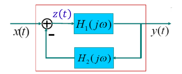
Consider a system with $x(t)$ as input. The error signal $e(t)$ is $x(t) + (-3y(t)) = x(t) - 3y(t)$. The block $D$ is a differentiator, so $y(t) = \frac{de(t)}{dt}$.
In the frequency domain:

$$\begin{cases} E(j\omega) = X(j\omega) - 3Y(j\omega) \\ Y(j\omega) = j\omega E(j\omega) \end{cases}$$

So,

$$Y(j\omega) = j\omega (X(j\omega)-3Y(j\omega)) \implies Y(j\omega) = j\omega X(j\omega) - 3j\omega Y(j\omega) \implies Y(j\omega)(1+3j\omega) = j\omega X(j\omega)$$

The frequency response is:

$$H(j\omega) = \frac{Y(j\omega)}{X(j\omega)} = \frac{j\omega}{1+3j\omega}$$

This can be rewritten using partial fractions:

$$H(j\omega) = \frac{j\omega}{3(j\omega + 1/3)} = \frac{1}{3} \frac{3j\omega}{3j\omega+1} = \frac{1}{3} \frac{ (3j\omega+1) - 1}{3j\omega+1} = \frac{1}{3}\left(1 - \frac{1}{1+3j\omega}\right) = \frac{1}{3} - \frac{1}{3} \frac{1}{1+3j\omega} = \frac{1}{3} - \frac{1}{9} \frac{1}{j\omega + 1/3}$$

The impulse response $h(t)$ is the IFT of $H(j\omega)$:

$$h(t) = \frac{1}{3}\delta(t) - \frac{1}{9}e^{-t/3}u(t)$$

---

Predicting Outputs for LCCDE Systems

• A system described by a Linear Constant-Coefficient Differential Equation (LCCDE) is an incrementally LTI system.

• The total response $y(t)$ is the sum of the zero-state response $y_{zs}(t)$ and the zero-input response $y_{zi}(t)$.

  $$y(t) = y_{zs}(t) + y_{zi}(t)$$

• The zero-state response is the output of an LTI subsystem and can be predicted in the frequency domain.

Generating Frequency Response from LCCDE

Given an LCCDE:

$$\sum_{k=0}^{N}a_{k}\frac{d^{k}y(t)}{dt^{k}} = \sum_{k=0}^{M}b_{k}\frac{d^{k}x(t)}{dt^{k}}$$

Apply Fourier transform to both sides. Using the differentiation property $\mathfrak{F}\left\{\frac{d^{k}f(t)}{dt^{k}}\right\} = (j\omega)^{k}F(j\omega)$:

$$\sum_{k=0}^{N}a_{k}(j\omega)^{k}Y(j\omega) = \sum_{k=0}^{M}b_{k}(j\omega)^{k}X(j\omega)$$

Rearranging for the frequency response $H(j\omega) = Y(j\omega)/X(j\omega)$ (this specifically gives the frequency response of the LTI subsystem for the zero-state response):

$$H(j\omega) = \frac{\sum_{k=0}^{M}b_{k}(j\omega)^{k}}{\sum_{k=0}^{N}a_{k}(j\omega)^{k}}$$

This is the general expression for the frequency response of a stable LCCDE system’s LTI part.

Example 4.25: Impulse Response of a 2nd-order LCCDE System
Given the LCCDE: $\frac{d^{2}y(t)}{dt^{2}}+4\frac{dy(t)}{dt}+3y(t)=\frac{dx(t)}{dt}+2x(t)$. Assume the system is stable.
Taking the Fourier transform:

$$(j\omega)^{2}Y(j\omega)+4(j\omega)Y(j\omega)+3Y(j\omega)=(j\omega)X(j\omega)+2X(j\omega)$$

$$[(j\omega)^{2}+4j\omega+3]Y(j\omega)=(j\omega+2)X(j\omega)$$

The frequency response is:

$$H(j\omega)=\frac{j\omega+2}{(j\omega)^{2}+4j\omega+3} = \frac{j\omega+2}{(j\omega+1)(j\omega+3)}$$

Using partial-fraction expansion:

$$H(j\omega)=\frac{A}{j\omega+1}+\frac{B}{j\omega+3}$$

$A(j\omega+3) + B(j\omega+1) = j\omega+2$.
If $j\omega = -1$, $A(-1+3) = -1+2 \Rightarrow 2A = 1 \Rightarrow A = 1/2$.
If $j\omega = -3$, $B(-3+1) = -3+2 \Rightarrow -2B = -1 \Rightarrow B = 1/2$.
So,

$$H(j\omega)=\frac{\frac{1}{2}}{j\omega+1}+\frac{\frac{1}{2}}{j\omega+3}$$

The impulse response (for the stable system) is:

$$h(t)=\frac{1}{2}e^{-t}u(t)+\frac{1}{2}e^{-3t}u(t)$$

Example 4.26: Output for a given input
For the same system, find the output $y(t)$ for $x(t)=e^{-t}u(t)$.
$X(j\omega) = \frac{1}{j\omega+1}$.
$Y(j\omega)=H(j\omega)X(j\omega)=\left[\frac{j\omega+2}{(j\omega+1)(j\omega+3)}\right]\left[\frac{1}{j\omega+1}\right] = \frac{j\omega+2}{(j\omega+1)^{2}(j\omega+3)}$.
Using partial-fraction expansion for repeated roots:

$$Y(j\omega)=\frac{A_{11}}{j\omega+1}+\frac{A_{12}}{(j\omega+1)^{2}}+\frac{A_{21}}{j\omega+3}$$

The coefficients are given as $A_{11}=\frac{1}{4}, A_{12}=\frac{1}{2}, A_{21}=-\frac{1}{4}$.
Thus, the zero-state response is:

$$y_{zs}(t)=\left[\frac{1}{4}e^{-t}+\frac{1}{2}te^{-t}-\frac{1}{4}e^{-3t}\right]u(t)$$

Caveats

1. Stability:

   1. To use this Fourier transform method for LCCDEs, we usually require the system to be stable.
   2. Stability (BIBO) implies $h(t)$ is absolutely integrable, which is a Dirichlet condition for the convergence of $H(j\omega)$.

2. Zero-State Response:

   1. This frequency response method directly predicts the zero-state response.
   2. If initial conditions are zero, or the system is LTI (implying initial rest for causality), then the full response is the zero-state response. Otherwise, the zero-input response must be solved separately (e.g., using the characteristic polynomial method).

Exercise: RC Circuit (Analog Lowpass Filter)

Consider an RC circuit with input voltage $V_{in}$ (or $v_s(t)$) across a series resistor R and capacitor C. The output voltage $V_{out}$ (or $v_c(t)$) is across the capacitor.
LCCDE: $RC\frac{dv_{c}(t)}{dt}+v_{c}(t)=v_{s}(t)$, which can be written as $\frac{dv_{c}(t)}{dt}+\frac{1}{RC}v_{c}(t)=\frac{1}{RC}v_{s}(t)$.
Frequency Response:
Taking FT: $RCj\omega V_{c}(j\omega)+V_{c}(j\omega)=V_{s}(j\omega)$.
$V_{c}(j\omega)(RCj\omega+1)=V_{s}(j\omega)$.

$$H(j\omega)=\frac{V_{c}(j\omega)}{V_{s}(j\omega)}=\frac{1}{1+RCj\omega}$$

Magnitude Spectrum:

$$|H(j\omega)|=\frac{1}{\sqrt{1+(RC\omega)^{2}}}$$

This system acts as an analog first-order lowpass filter. It allows low-frequency signals to pass while attenuating high-frequency signals.

---

Multiplication Property

The multiplication property is dual to the convolution property.
If $s(t)\leftrightarrow S(j\omega)$ and $p(t)\leftrightarrow P(j\omega)$, then:

$$r(t)=s(t) \cdot p(t)\leftrightarrow R(j\omega)=\frac{1}{2\pi}[S(j\omega)*P(j\omega)]$$

Multiplication in the time domain corresponds to convolution in the frequency domain (scaled by $1/(2\pi)$).

Proof (using duality)

1. Given $s(t)\leftrightarrow S(\omega)$ and $p(t)\leftrightarrow P(\omega)$.
2. By duality, $S(t)\leftrightarrow 2\pi s(-\omega)$ and $P(t)\leftrightarrow 2\pi p(-\omega)$.
3. Using the convolution property: $S(t)*P(t)\leftrightarrow (2\pi s(-\omega))(2\pi p(-\omega)) = 4\pi^{2}s(-\omega)p(-\omega)$.
4. Let $g(t) = S(t)*P(t)$ and $G(\omega) = 4\pi^{2}s(-\omega)p(-\omega)$.
5. Applying duality again to $g(t) \leftrightarrow G(\omega)$: $G(t) \leftrightarrow 2\pi g(-\omega)$.
   $4\pi^{2}s(-t)p(-t) \leftrightarrow 2\pi [S(-\omega)*P(-\omega)]$.
   Replacing $t$ with $-t$: $4\pi^{2}s(t)p(t) \leftrightarrow 2\pi [S(\omega)*P(\omega)]$ (assuming $S$ and $P$ are transforms from $t \to \omega$, so the convolution arguments become $\omega$).
   Therefore, $s(t)p(t) \leftrightarrow \frac{1}{2\pi}[S(j\omega)*P(j\omega)]$.

Example 4.23: FT of a product of sinc functions
Find the Fourier transform of

$$x(t)=\frac{\sin(t)\sin(t/2)}{\pi t^{2}}$$

Rewrite $x(t)$ as:

$$x(t)=\pi\left(\frac{\sin(t)}{\pi t}\right)\left(\frac{\sin(t/2)}{\pi t}\right)$$

Let $s_1(t) = \frac{\sin(t)}{\pi t}$ and $s_2(t) = \frac{\sin(t/2)}{\pi t}$.

We know that

$$\mathfrak{F}\{\frac{\sin(Wt)}{\pi t}\} = \text{rect}(\frac{\omega}{2W}) = \begin{cases} 1, & |\omega| < W \\ 0, & |\omega| > W \end{cases}$$

So, $S_1(j\omega) = \text{rect}(\frac{\omega}{2})$ (i.e., 1 for $|\omega|<1$, 0 otherwise).
And $S_2(j\omega) = \text{rect}(\omega)$ (i.e., 1 for $|\omega|<1/2$, 0 otherwise, because $W=1/2$).

$$X(j\omega) = \pi \cdot \frac{1}{2\pi} [S_1(j\omega) * S_2(j\omega)] = \frac{1}{2}[S_1(j\omega) * S_2(j\omega)]$$

This is the convolution of two rectangular functions.
$S_1(j\omega)$ is a rectangle from $\omega=-1$ to $1$ with height 1.
$S_2(j\omega)$ is a rectangle from $\omega=-1/2$ to $1/2$ with height 1.
The convolution of these two rectangular pulses will result in a trapezoidal（梯形） pulse.
The convolution will range from $(-1 - 1/2)$ to $(1 + 1/2)$, i.e., from $-3/2$ to $3/2$.
The flat top will be from $(-1+1/2)$ to $(1-1/2)$, i.e., from $-1/2$ to $1/2$. The height of the convolution is Area($S_2(j\omega)$) = $1 \times 1 = 1$.
So $X(j\omega)$ will be a trapezoid with:

• Value $0$ for $\omega < -3/2$ and $\omega > 3/2$.
• Linearly increasing from $0$ at $\omega=-3/2$ to $1/2 \times 1 = 1/2$ at $\omega=-1/2$.
• Constant value $1/2$ for $-1/2 \le \omega \le 1/2$.
• Linearly decreasing from $1/2$ at $\omega=1/2$ to $0$ at $\omega=3/2$.

---

Modulation and Demodulation

Modulation System (Example 4.21)

Assume a bandlimited signal $s(t)$ with spectrum $S(j\omega)$ (bandlimited to $\omega_1$, i.e., $S(j\omega)=0$ for $|\omega| > \omega_1$).
Multiply $s(t)$ with a high-frequency sinusoidal function $p(t) = \cos(\omega_0 t)$, where $\omega_0 \gg \omega_1$.
The Fourier transform of $p(t)=\cos(\omega_0 t)$ is $P(j\omega) = \pi[\delta(\omega-\omega_0) + \delta(\omega+\omega_0)]$.
The resulting signal is $r(t) = s(t)p(t)$.
Its spectrum $R(j\omega)$ is given by the multiplication property:

$$R(j\omega) = \frac{1}{2\pi}[S(j\omega) * P(j\omega)]$$

$$R(j\omega) = \frac{1}{2\pi}[S(j\omega) * (\pi[\delta(\omega-\omega_0) + \delta(\omega+\omega_0)])]$$

$$R(j\omega) = \frac{1}{2}[S(j\omega) * \delta(\omega-\omega_0) + S(j\omega) * \delta(\omega+\omega_0)]$$

Using the sifting property of convolution with an impulse:

$$S(j\omega) * \delta(\omega-\omega_c) = S(j(\omega-\omega_c))$$

$$R(j\omega) = \frac{1}{2}[S(j(\omega-\omega_0)) + S(j(\omega+\omega_0))]$$

This means the original spectrum $S(j\omega)$ is shifted to $\pm\omega_0$ and scaled by $1/2$. This is amplitude modulation.

Demodulation System (Example 4.22)

（同步解调）

To recover the original signal $s(t)$ from the modulated signal $r(t)$:

1. Multiply $r(t)$ with $p(t) = \cos(\omega_0 t)$ again:
   • Let $g(t) = r(t)p(t)$.
     $G(j\omega) = \frac{1}{2\pi}[R(j\omega) * P(j\omega)]$
     $R(j\omega)$ has components centered at $\pm\omega_0$. $P(j\omega)$ has impulses at $\pm\omega_0$.
   • Convolution will result in:
     $G(j\omega) = \frac{1}{2}[R(j(\omega-\omega_0)) + R(j(\omega+\omega_0))]$
   • Substituting $R(j\omega) = \frac{1}{2}[S(j(\omega-\omega_0)) + S(j(\omega+\omega_0))]$:
     $G(j\omega) = \frac{1}{2} \left[ \frac{1}{2}(S(j(\omega-2\omega_0)) + S(j\omega)) + \frac{1}{2}(S(j\omega) + S(j(\omega+2\omega_0))) \right]$
     $G(j\omega) = \frac{1}{2}S(j\omega) + \frac{1}{4}S(j(\omega-2\omega_0)) + \frac{1}{4}S(j(\omega+2\omega_0))$
   • The spectrum $G(j\omega)$ contains the original baseband spectrum $S(j\omega)$ (scaled by $1/2$) centered at $\omega=0$, plus copies centered at $\pm 2\omega_0$.
2. Apply a Lowpass Filter:
   • Pass $g(t)$ through a lowpass filter $H_{LPF}(j\omega)$ that keeps frequencies up to $\omega_1$ (and removes components around $\pm 2\omega_0$).
   • The output will be $\frac{1}{2}S(j\omega)$, which is a scaled version of the original signal’s spectrum.
   • This modulation/demodulation process is invertible.

---

Wireless Transmission (Frequency Division Multiplexing)

Modulation is used in wireless transmission to send multiple signals over the same channel by modulating them onto different carrier frequencies.

• Transmitter Side: Multiple signals (e.g., voices) are modulated using different carrier frequencies (e.g., $\cos(2\pi f_1 t)$, $\cos(2\pi f_2 t)$, etc.). The modulated signals are then added together. In the frequency domain, their spectra are shifted to different frequency bands and do not overlap.
• Receiver Side: To recover a specific signal (e.g., signal 1):
  1. Multiply the combined received signal by the corresponding carrier frequency (e.g., $\cos(2\pi f_1 t)$). This shifts the desired signal’s spectrum back to baseband (around $\omega=0$) and other signals to other frequencies.
  2. Apply a lowpass filter to extract the baseband signal, recovering the original signal.
     This technique is known as Amplitude Modulation (AM).

---

Generating a Bandpass Filter from a Lowpass Filter

A bandpass filter can be created from an ideal lowpass filter $H_{LP}(j\omega)$ (with cutoff $\omega_c$) using modulation.

1. Let the input signal be $x(t)$ and its spectrum $X(j\omega)$.
2. Modulate the input signal: $x(t)e^{j\omega_c t}$. Its spectrum is $X(j(\omega-\omega_c))$.
3. Pass this through the lowpass filter $H_{LP}(j\omega)$. The output spectrum is $H_{LP}(j\omega)X(j(\omega-\omega_c))$. This is a version of $X(j\omega)$ that was originally around $\omega_c$, now shifted to baseband and filtered.
4. Take the real part of the output signal

$$\mathfrak{Re} \{f(t)\} = \frac{f(t) + f^*(t)}{2} \stackrel{\mathcal{F}}{\rightarrow} \frac{F(j\omega) + F^*(-j\omega)}{2}$$

To create a bandpass filter centered at $\omega_c$:

• Consider an ideal lowpass filter $H_{LP}(j\omega)$ which is 1 for $|\omega| < \omega_0$ and 0 otherwise.
• The frequency response of an ideal bandpass filter centered at $\pm\omega_c$ with bandwidth $2\omega_0$ can be thought of as

$$H_{BP}(j\omega) = H_{LP}(j(\omega-\omega_c)) + H_{LP}(j(\omega+\omega_c))$$

• Alternatively, to create a real bandpass filter $h_{BP}(t)$ from a real lowpass filter $h_{LP}(t)$:

$$h_{BP}(t) = 2h_{LP}(t)\cos(\omega_c t)$$

• In the frequency domain:

$$H_{BP}(j\omega) = H_{LP}(j(\omega-\omega_c)) + H_{LP}(j(\omega+\omega_c))$$

• This effectively shifts the lowpass response to $\pm\omega_c$.