Chapter9 Laplace Transform

Lecture 13 - Laplace Transform and Inverse Laplace Transform

Motivation for Laplace Transform 💡

• The Fourier Transform is a powerful tool, but it has limitations.
• A key Dirichlet condition for the convergence of the Fourier Transform is that the signal must be absolutely integrable ($\int_{-\infty}^{\infty} |x(t)| dt < \infty$).
• Signals like $x(t)=e^{t}u(t)$ are not absolutely integrable, and their Fourier Transform would result in infinities.
• Fourier analysis is suitable for absolutely integrable signals and stable LTI systems (whose impulse response is absolutely integrable). For other signals and systems, it’s not guaranteed to work.
• The Laplace Transform is a more generalized tool that can handle non-absolutely-integrable signals and unstable systems.

---

The Laplace Transform: Definition 📜

For an arbitrary signal $x(t)$, its Laplace Transform $X(s)$ is defined as:

$$X(s) = \mathfrak{L}\{x(t)\} \triangleq \int_{-\infty}^{\infty} x(t)e^{-st} dt$$

where $s = \sigma + j\omega$ is a complex variable.

• Note: The Fourier Transform is a special case of the Laplace Transform when $\sigma = 0$ (i.e., on the $j\omega$ axis in the s-plane).
  $X(j\omega) = \int_{-\infty}^{\infty} x(t)e^{-j\omega t} dt$.
• The Laplace transform can be viewed as a 2-dimensional continuous-time signal on the s-plane.

---

A Set of “Preconditioned” Fourier Transforms

The Laplace Transform can be interpreted as the Fourier Transform of a “preconditioned” signal.
Let $s = \sigma + j\omega$. Then,

$$X(s) = \int_{-\infty}^{\infty} x(t)e^{-\sigma t}e^{-j\omega t} dt = \int_{-\infty}^{\infty} [x(t)e^{-\sigma t}]e^{-j\omega t} dt = \mathfrak{F}\{x(t)e^{-\sigma t}\}$$

The term $x(t)e^{-\sigma t}$ is the preconditioned signal.

• For $\sigma = 0$, $X(s)$ is directly the Fourier Transform of $x(t)$.
• For $\sigma \neq 0$, the Laplace Transform of $x(t)$ is the Fourier Transform of the preconditioned signal $x(t)e^{-\sigma t}$.
• Although $x(t)$ might not satisfy the 1st Dirichlet condition, $x(t)e^{-\sigma t}$ may satisfy it for certain values of $\sigma$. This “preconditioning” allows analysis of signals not representable by the Fourier Transform.

Example: $x(t) = e^{t}u(t)$
This signal is not absolutely integrable, so its Fourier Transform doesn’t converge in the usual sense.
However, the preconditioned signal is $e^{t}u(t) \cdot e^{-\sigma t} = e^{-(\sigma-1)t}u(t)$.

• This preconditioned signal is representable by FT if $\sigma-1 > 0$ (i.e., $\sigma > 1$), as the growing exponential is changed into a decaying one.
• It is not representable by FT if $\sigma-1 \le 0$.
  Thus, even if the FT of the original signal doesn’t converge, the FT of the preconditioned signal might, allowing the Laplace Transform to be used.

---

Region of Convergence (ROC) 🌐

• The Laplace Transform of a signal often converges for some values of $\sigma$ but not for others.
• The Region of Convergence (ROC) is the set of all points $s$ in the s-plane for which the Laplace Transform integral is finite:

  $$ROC = \{s \in \mathbb{C} | |\mathfrak{L}\{x(t)\}(s)| < \infty \}$$

• The ROC is often visualized as a shaded area in a “bird-view” of the s-plane.

Example: Evaluate the Laplace Transform of $x(t) = e^{-at}u(t)$ and its ROC.

$$X(s) = \int_{-\infty}^{\infty} e^{-at}u(t)e^{-st} dt = \int_{0}^{\infty} e^{-(s+a)t} dt$$

Let $s = \sigma + j\omega$. Then the integral becomes

$$X(s) = \int_{0}^{\infty} e^{-(\sigma+a)t}e^{-j\omega t} dt = \mathfrak{F}\{e^{-(\sigma+a)t}u(t)\}$$

• If $\sigma+a > 0$, or $Re\{s\} > -a$, then $X(s) = \frac{1}{j\omega + \sigma + a} = \frac{1}{s+a}$.
• Otherwise, if $Re\{s\} \le -a$, the integral is $\infty$.
• Thus, the Laplace Transform is $X(s) = \frac{1}{s+a}$, with the ROC: $Re\{s\} > -a$. We write it as

$$X(s) = \frac{1}{s+a} ; Re\{s\} > -a$$

Caveat on ROC:

• $X(s) = \frac{1}{s+a}; Re\{s\} > -a$ actually means:

$$X(s) = \begin{cases} \frac{1}{s+a}; & Re\{s\} > -a \\ \infty; & Re\{s\} \le -a \end{cases}$$

• This is not equivalent to $X(s) = \frac{1}{s+a}; Re\{s\} < -a$. They represent different functions.
• Two different functions can have an identical algebraic expression for their Laplace Transform but different ROCs.
  • $x(t) = e^{-at}u(t) \implies X(s) = \int_0^\infty e^{-(s+a)t} dt = \frac{1}{s+a}$, ROC: $Re\{s\} > -a$.
  • $x(t) = -e^{-at}u(-t) \implies X(s) = -\int_{-\infty}^0 e^{-(s+a)t} dt = \frac{1}{s+a}$, ROC: $Re\{s\} < -a$.
• You must present both the algebraic form and the ROC for a complete description of the Laplace Transform.

Example [Example 9.3]: Determine the Laplace Transform (including ROC) of $x(t) = 3e^{-2t}u(t) - 2e^{-t}u(t)$.

$$X(s) = \int_{-\infty}^{\infty} [3e^{-2t}u(t) - 2e^{-t}u(t)]e^{-st} dt X(s) = 3\int_{0}^{\infty} e^{-(s+2)t}dt - 2\int_{0}^{\infty} e^{-(s+1)t}dt$$

• The first term is $\frac{3}{s+2}$ with ROC $Re\{s\} > -2$.
• The second term is $\frac{2}{s+1}$ with ROC $Re\{s\} > -1$.
• For $X(s) = \frac{3}{s+2} - \frac{2}{s+1}$ to be valid, both ROCs must be satisfied. The overall ROC is the intersection of the individual ROCs.
• Thus, $X(s) = \frac{3}{s+2} - \frac{2}{s+1}$, with ROC: $Re\{s\} > -1$.

Using ROC to determine convergence of FT:

• If the ROC of the Laplace Transform includes the $j\omega$ axis ($Re\{s\}=0$), then the Fourier Transform $X(0+j\omega) = \mathfrak{F}\{x(t)\}$ converges.
• Otherwise, if the ROC does not include the $j\omega$ axis, the Fourier Transform does not converge.

---

Pole-Zero Plot (零极点图) 🗺️

• The Laplace Transform is often visualized with a bird’s-eye view of the s-plane. This view makes ROC specification easy. However, it’s not great for showing the value of $X(s)$ itself.
• Zeros (零点): Values of $s$ for which $X(s) = 0$.
• Poles (极点): Values of $s$ for which $X(s) = \infty$.
• Zeros and poles can be complex-valued.

Example: Let $X(s) = \frac{s-1}{(s+2)(s+1)}$; ROC: $Re\{s\} > -1$.

• Zero: $s=1$.
• Poles: $s=-1, s=-2$.

A pole-zero plot adds labels for zeros (often ‘o’) and poles (often ‘x’) to the s-plane view, giving a rough understanding of the magnitude of $X(s)$.

Virtual Poles/Zeros for Rational Laplace Transform

Consider $X(s) = \frac{N(s)}{D(s)}$, where N(s) and D(s) are polynomials in s.

• If Order(D) > Order(N) $\implies X(\infty) = 0 \implies$ virtual zeros at $s=\infty$. (e.g., $\frac{1}{s+1}$)
• If Order(D) < Order(N) $\implies X(\infty) = \infty \implies$ virtual poles at $s=\infty$. (e.g., $s+1$)
• If Order(D) = Order(N) $\implies$ neither zeros nor poles exist at $s=\infty$.
• Example: For $X(s) = \frac{s-1}{(s+2)(s+1)}$, Order(D) = 2, Order(N) = 1. So, there is a virtual zero at $s=\infty$. It has two poles at $s=-2$ & $s=-1$, and two zeros at $s=1$ & $s=\infty$.

Poles/Zeros for Rational Laplace Transform - Caveat

For rational Laplace transforms

$$X(s) = \frac{N(s)}{D(s)} = M\frac{\prod (s-\beta_n)}{\prod (s-\alpha_i)}$$

poles are usually the roots of the denominator $D(s)$, and zeros are usually the roots of the numerator $N(s)$.

• HOWEVER, this is not true in general. Exceptions occur when the numerator and denominator share a common root.

Example: $x(t) = e^{-at}$ for $0 < t < T$, and $0$ otherwise.

$$X(s) = \int_{0}^{T} e^{-at}e^{-st}dt = \int_{0}^{T} e^{-(s+a)t}dt = \frac{1}{s+a}[1 - e^{-(s+a)T}]$$

• It looks like $s=-a$ is a pole.
• No, $s=-a$ is a root of both the numerator (as $1-e^{-(-a+a)T} = 1-e^0 = 0$) and the denominator.
• Using L’Hospital’s rule for $s \to -a$:

$$\lim_{s \to -a} \frac{1-e^{-(s+a)T}}{s+a} = \lim_{s \to -a} \frac{-(-T)e^{-(s+a)T}}{1} = Te^0 = T$$

• So, $X(-a) = T$, which means $s=-a$ is neither a pole nor a zero.
• A “zero” and “pole” at the same location in the s-plane may cancel each other out.
• We can’t determine poles and zeros simply by roots of the denominator and numerator; we need to judge based on the value of $X(s)$!

Computer-aided visualization: Plotting $|X(s)|$ or $\angle X(s)$ on the s-plane (e.g., using MATLAB) can provide a more complete picture than just the pole-zero plot.

---

Properties of ROC 📌

The ROC for a Laplace transform obeys certain rules:

Property #1: The ROC of $X(s)$ consists of vertical strips parallel to the $j\omega$-axis in the s-plane.

• If a point $s_0$ is in the ROC, then the entire line $\{s_0 + j\omega | \omega \in \mathbb{R}\}$ is in the ROC.
• If a point $s_0 \notin \text{ROC}$, then the entire line $\{s_0 + j\omega | \omega \in \mathbb{R}\} \not\subset \text{ROC}$
• This is because the convergence depends on $\mathfrak{F}\{x(t)e^{-\sigma t}\}$. If this Fourier Transform converges for a given $\sigma$, it converges for all $\omega$ associated with that $\sigma$. Thus, ROC membership is independent of $\omega$.

Property #2: The ROC does not contain any poles (and thus, the vertical lines passing through the poles are not in the ROC).

• If $s_0$ is a pole, $X(s_0) = \infty$, so $s_0$ is not in the ROC. By Property #1, the entire vertical line through $s_0$ is not in the ROC.

Property #3: If $x(t)$ is of finite duration and absolutely integrable (i.e., $\int_{T_1}^{T_2} |x(t)|dt < \infty$ for $x(t)$ non-zero only in $T_1 \le t \le T_2$), then the ROC is the entire s-plane.

• *Proof *: $\int_{T_1}^{T_2} |x(t)e^{-\sigma t}|dt = \int_{T_1}^{T_2} |x(t)||e^{-\sigma t}|dt$.
  • Since $e^{-\sigma t}$ is bounded over any finite interval $[T_1, T_2]$ for any finite $\sigma$,
  • if $\int_{T_1}^{T_2} |x(t)|dt < \infty$, then $\int_{T_1}^{T_2} |x(t)e^{-\sigma t}|dt \le \max(|e^{-\sigma T_1}|, |e^{-\sigma T_2}|) \int_{T_1}^{T_2} |x(t)|dt < \infty$ for all $\sigma$.

Property #4: If $x(t)$ is a right-sided signal (i.e., $x(t)=0$ for $t<T$ ), and if a line $Re\{s\}=\sigma_0$ is in the ROC, then all values of $s$ for which $Re\{s\} > \sigma_0$ are also in the ROC.

• The ROC is a right half-plane bounded by some $\sigma_R$ that satisfies $\sigma_R < \sigma_0$ , possibly $\mathbb{C}$.
• The factor $e^{-\sigma t}$ provides increasing attenuation for $t>0$ as $\sigma$ increases, aiding convergence for large $t$.

Property #5: If $x(t)$ is a left-sided signal (i.e., $x(t)=0$ for $t>T_2$ for some $T_2$), and if a line $Re\{s\}=\sigma_0$ is in the ROC, then all values of $s$ for which $Re\{s\} < \sigma_0$ are also in the ROC.

• The ROC is a left half-plane bounded by some $\sigma_L$ that satisfies $\sigma_L > \sigma_0$ , possibly $\mathbb{C}$.
• The factor $e^{-\sigma t}$ provides decreasing attenuation (or increasing gain) for $t<0$ as $\sigma$ decreases (becomes more negative), aiding convergence for large negative $t$.

Property #6: If $x(t)$ is a two-sided signal（双边都有，即无限信号）, and if a line $Re\{s\}=\sigma_0$ is in the ROC, then the ROC is a vertical strip in the s-plane that includes $Re\{s\}=\sigma_0$. It can also be empty or, if $x(t)$ is finite duration, the entire s-plane.

• A two-sided signal can be written as $x(t) = x_R(t) + x_L(t)$, where $x_R(t)$ is right-sided and $x_L(t)$ is left-sided.
• The ROC of $X(s)$ is the intersection of the ROC of $X_R(s)$ (a right half-plane $Re\{s\} > \sigma_R$) and the ROC of $X_L(s)$ (a left half-plane $Re\{s\} < \sigma_L$).
  • If $\sigma_R < \sigma_L$, the intersection is the strip $\sigma_R < Re\{s\} < \sigma_L$.
  • Else, the intersection is empty, which means the ROC is empty
  • If both ROCs are the entire s-plane, then the intersection is the entire s-plane.

Summary of ROC shapes based on signal type:

Signal Type	Typical ROC Shape
Finite Duration (Compact Support)	Entire s-plane (if absolutely integrable) or empty
Right-sided	Right half-plane ($Re\{s\} > \sigma_{max}$) or empty
Left-sided	Left half-plane ($Re\{s\} < \sigma_{min}$) or empty
Two-sided (Infinite) （双边都有，即无限信号）	Single Vertical strip ($\sigma_1 < Re\{s\} < \sigma_2$) or empty

Example 9.7: $x(t) = e^{-b|t|}$
This is a two-sided signal: $x(t) = e^{-bt}u(t) + e^{bt}u(-t)$.

• For $e^{-bt}u(t)$, $X_1(s) = \frac{1}{s+b}$, ROC: $Re\{s\} > -b$.
• For $e^{bt}u(-t)$, $X_2(s) = \frac{-1}{s-b}$, ROC: $Re\{s\} < b$.
  The ROC for $X(s)$ is the intersection of these two ROCs.
• If $b>0$: $-b < Re\{s\} < b$. The Laplace Transform is $X(s) = \frac{1}{s+b} - \frac{1}{s-b} = \frac{-2b}{s^2-b^2}$.
• If $b<0$: Let $b' = -b > 0$. Then $x(t) = e^{b'|t|}$. The ROCs are $Re\{s\} > b'$ and $Re\{s\} < -b'$. Since $b' > 0$, there is no common area, so the Laplace Transform does not converge for any $s$.
• If $b=0$: $x(t)=1$. This is not absolutely integrable, and the Laplace transform does not converge (except in generalized function sense, which is beyond this scope).

---

Properties of ROC for Rational Laplace Transforms

For Laplace Transforms $X(s)$ that are rational functions of $s$ (i.e., a ratio of polynomials in $s$):

Property #7: If the Laplace Transform $X(s)$ of $x(t)$ is rational, then its ROC is bounded by poles or extends to infinity.
This means the ROC is a vertical strip (or half-plane) whose boundaries are defined by the real parts of poles.

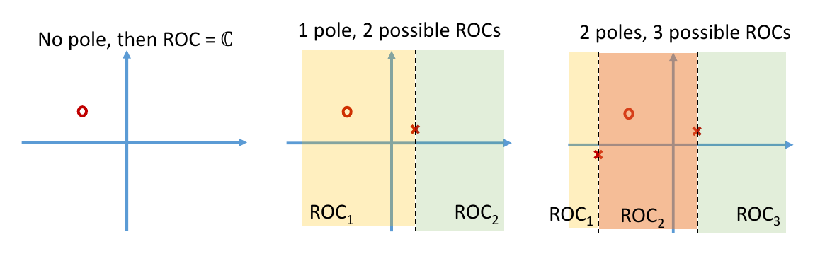
• No poles: ROC is the entire s-plane.
• 1 pole at $s=p_1$: ROC is $Re\{s\} > Re\{p_1\}$ or $Re\{s\} < Re\{p_1\}$. (2 possible ROCs)
• 2 poles at $s=p_1, s=p_2$ (assume $Re\{p_1\} < Re\{p_2\}$): ROC is $Re\{s\} < Re\{p_1\}$, or $Re\{p_1\} < Re\{s\} < Re\{p_2\}$, or $Re\{s\} > Re\{p_2\}$. (3 possible ROCs)

Property #8: If $X(s)$ is rational and its ROC exists (i.e., it converges for at least one point):

• If $x(t)$ is right-sided, the ROC is the region in the s-plane to the right of the rightmost pole (i.e., $Re\{s\} > \max(Re\{p_i\})$). This is more specific than Property #4.
• If $x(t)$ is left-sided, the ROC is the region in the s-plane to the left of the leftmost pole (i.e., $Re\{s\} < \min(Re\{p_i\})$). This is more specific than Property #5.
• If $x(t)$ is two-sided, the ROC is a single strip between two adjacent poles (i.e., $Re\{p_k\} < Re\{s\} < Re\{p_j\}$ for some poles $p_k, p_j$, and no poles exist in this strip). This is more specific than Property #6.

Invalid ROC examples based on properties:

• A ROC that includes a pole violates Property #2.
• A ROC for a rational transform that is not bounded by poles (e.g., a finite, non-strip region, or a strip whose boundaries are not poles) violates Property #7.
• A ROC for a right-sided signal that is to the left of a pole, or a left-sided signal to the right of a pole, or a two-sided signal that is not between two poles (or is a half-plane) violates Property #8.

Example 9.8: Determine all possible ROCs and corresponding signal types for $X(s) = \frac{1}{s^2+3s+2} = \frac{1}{(s+1)(s+2)}$.
This can be written using partial fractions as $X(s) = \frac{1}{s+1} - \frac{1}{s+2}$.
The poles are at $s=-1$ and $s=-2$.
Since $X(s)$ is rational, there are 3 possible ROCs based on Property #7 & #8:

1. ROC1: $Re\{s\} > -1$. This is a right half-plane bounded by the rightmost pole ($s=-1$). This indicates $x(t)$ is a right-sided signal.

   $$x(t) = (e^{-t} - e^{-2t})u(t)$$

2. ROC2: $Re\{s\} < -2$. This is a left half-plane bounded by the leftmost pole ($s=-2$). This indicates $x(t)$ is a left-sided signal.

   $$x(t) = (-e^{-t} + e^{-2t})u(-t)$$

3. ROC3: $-2 < Re\{s\} < -1$. This is a strip between two adjacent poles. This indicates $x(t)$ is a two-sided signal.

   $$x(t) = -e^{-t}u(-t) - e^{-2t}u(t)$$

Supplement

Exact Number of zeros and poles at $\infty$

Here’s how to determine the specific number for a rational Laplace Transform $X(s) = \frac{N(s)}{D(s)}$:

Let $M$ be the degree (highest power of $s$) of the numerator polynomial $N(s)$.
Let $K$ be the degree of the denominator polynomial $D(s)$.

The behavior at $s=\infty$ depends on the relative degrees of these polynomials:

1. If the degree of the denominator is greater than the degree of the numerator ($K > M$):

   • $X(s)$ approaches $0$ as $s \to \infty$.
   • There are $K-M$ zeros at $s=\infty$.

2. If the degree of the numerator is greater than the degree of the denominator ($M > K$):

   • $X(s)$ approaches $\infty$ as $s \to \infty$.
   • There are $M-K$ poles at $s=\infty$.

3. If the degree of the numerator is equal to the degree of the denominator ($M = K$):

   • $X(s)$ approaches a finite, non-zero constant as $s \to \infty$.
   • There are neither poles nor zeros at $s=\infty$.

Essentially, you’re looking at how $X(s)$ behaves as $s$ becomes very large. For large $s$, $X(s) \approx \frac{a_M s^M}{b_K s^K} = \frac{a_M}{b_K} s^{M-K}$. The exponent $M-K$ tells you the nature and number of roots at infinity:

• If $M-K$ is negative (i.e., $K-M$ is positive), you have $K-M$ zeros at infinity.
• If $M-K$ is positive, you have $M-K$ poles at infinity.
• If $M-K$ is zero, no poles or zeros at infinity.

Lecture 14: Properties of Laplace Transform

These notes cover the remaining properties of the Region of Convergence (ROC), the Inverse Laplace Transform, and the algebraic properties of the Laplace Transform.

---

Properties of ROC

The Region of Convergence (ROC) for the Laplace transform has several defining properties. These properties help in understanding the characteristics of the signal $x(t)$ from its Laplace transform $X(s)$.

Basic Properties of ROC

• Different types of signals have different ROCs. These include:
  • Compactly supported signals
  • Right-sided signals
  • Left-sided signals
  • Two-sided signals

Properties of ROC for Rational Laplace Transform

Property #7

• If the Laplace transform $X(s)$ of $x(t)$ is rational, then its ROC is bounded by poles or extends to infinity.
• This property helps determine the ROC for a rational Laplace transform spectrum.
  • If there are no poles, the ROC is the entire s-plane ($\mathbb{C}$).
  • With 1 pole, there are 2 possible ROCs (e.g., $Re\{s\} > \sigma_1$ or $Re\{s\} < \sigma_1$).
  • With 2 poles, there are 3 possible ROCs (e.g., $Re\{s\} < \sigma_1$, $\sigma_1 < Re\{s\} < \sigma_2$, or $Re\{s\} > \sigma_2$).
• Some ROC configurations are impossible as they violate basic ROC properties (like Property #2, which states ROC consists of strips parallel to the $j\omega$-axis) or properties #7 and #8.

Property #8
If the Laplace transform $X(s)$ of $x(t)$ is rational and converges for at least one point in the s-plane:

• If $x(t)$ is right-sided, the ROC is the right half-plane bounded by the rightmost pole. This is more specific than the general Property #4 for right-sided signals.
• If $x(t)$ is left-sided, the ROC is the left half-plane bounded by the leftmost pole. This is more specific than the general Property #5 for left-sided signals.
• If $x(t)$ is two-sided, the ROC is a single strip between two adjacent poles. This is more specific than the general Property #6 for two-sided signals.

---

Example 9.8: Determining ROCs and Signal Types

Given the Laplace transform:

$$X(s) = \frac{1}{s^2 + 3s + 2} = \frac{1}{s+1} - \frac{1}{s+2}$$

Steps to analyze:

1. Is this rational? Yes.
2. What are the poles? The poles are at $s = -1$ and $s = -2$.
3. Use Property #8.

Since $X(s)$ is rational, there are 3 possible ROCs and corresponding signal types:

• ROC1: $Re\{s\} > -1$. This is a right half-plane bounded by the rightmost pole (s=-1), indicating $x(t)$ is a right-sided signal.
• ROC2: $Re\{s\} < -2$. This is a left half-plane bounded by the leftmost pole (s=-2), indicating $x(t)$ is a left-sided signal.
• ROC3: $-2 < Re\{s\} < -1$. This is a strip between two adjacent poles, indicating $x(t)$ is a two-sided signal.

---

Inverse Laplace Transform (拉普拉斯反变换)

The Laplace transform can be inverted to retrieve the time-domain signal $x(t)$ from its s-domain representation $X(s)$.

• Laplace transform: $x(t) \rightarrow X(s)$
• Inverse Laplace transform: $X(s) \rightarrow x(t)$

Theoretical Formula for Inverse Laplace Transform

The inverse Laplace transform is defined by the line integral:

$$x(t) = \frac{1}{2\pi j} \int_{\sigma-j\infty}^{\sigma+j\infty} X(s)e^{st}ds$$

where the integration is performed along a line $Re\{s\} = \sigma$ within the ROC of $X(s)$.

Proof of Inverse Laplace Transform Formula

The proof is based on the relationship $X(s) = X(\sigma + j\omega) = \mathfrak{F}\{x(t)e^{-\sigma t}\}$, where $\mathfrak{F}$ denotes the Fourier Transform.
For any $\sigma$ in the ROC:
$x(t)e^{-\sigma t} = \mathfrak{F}^{-1}\{X(\sigma+j\omega)\} = \frac{1}{2\pi} \int_{-\infty}^{+\infty} X(\sigma+j\omega)e^{j\omega t}d\omega$
This leads to:
$x(t) = e^{\sigma t} \cdot \frac{1}{2\pi} \int_{-\infty}^{+\infty} X(\sigma+j\omega)e^{j\omega t}d\omega$
$x(t) = \frac{1}{2\pi} \int_{-\infty}^{+\infty} X(\sigma+j\omega)e^{(\sigma+j\omega)t}d\omega$
Let $s = \sigma + j\omega$, so $ds = j d\omega$. When $\omega \rightarrow \pm\infty$, $s \rightarrow \sigma \pm j\infty$.
$x(t) = \frac{1}{2\pi j} \int_{\sigma-j\infty}^{\sigma+j\infty} X(s)e^{st}ds$

Notes on Inverse Laplace Transform:

• The formula $x(t) = \frac{1}{2\pi j}\int_{\sigma-j\infty}^{\sigma+j\infty}X(s)e^{st}ds$ is based on $x(t)=e^{\sigma t}\mathfrak{F}^{-1}\{X(\sigma+j\omega)\}$ for $\sigma \in ROC$.
• The line of integration ($Re\{s\} = \sigma$) must belong to the ROC.
• Any line (any $\sigma$) within the ROC can be used to evaluate the inverse Laplace transform, and all will yield the same result.

---

Practical Evaluation Method for Inverse Laplace Transform (PROCS)

Direct inversion using the line integral can be difficult. For rational Laplace transforms, the PROCS procedure is often easier:

1. Partial-fraction expansion of $X(s)$.
2. Determine the ROC of each fraction based on the overall ROC of $X(s)$.
3. Determine the Signal of each fraction using a table of common Laplace transform pairs (like Table 9.2).

Table 9.2 (Selected Pairs):

Transform Pair	Signal $x(t)$	Transform $X(s)$	ROC
2	$u(t)$	$\frac{1}{s}$	$Re\{s\}>0$
3	$-u(-t)$	$\frac{1}{s}$	$Re\{s\}<0$
6	$e^{-\alpha t}u(t)$	$\frac{1}{s+\alpha}$	$Re\{s\}>-\alpha$
7	$-e^{-\alpha t}u(-t)$	$\frac{1}{s+\alpha}$	$Re\{s\}<-\alpha$
8	$[\cos \omega_0 t]u(t)$	$\frac{s}{s^2+\omega_0^2}$	$\text{Re}\{s\} > 0$
9	$[\sin \omega_0 t]u(t)$	$\frac{\omega_0}{s^2+\omega_0^2}$	$\text{Re}\{s\} > 0$

---

Examples 9.9-9.11: PROCS Procedure

Determine the original signal $x(t)$ for $X(s) = \frac{1}{(s+1)(s+2)}$ with different ROCs.
Partial-fraction expansion: $X(s) = \frac{1}{s+1} - \frac{1}{s+2}$.

1. Case 1: ROC is $Re\{s\} > -1$

   • P step: $X(s) = \frac{1}{s+1} - \frac{1}{s+2}$.
   • ROC step:
     • For the term $\frac{1}{s+1}$ (pole at $s=-1$): ROC must be $Re\{s\} > -1$.
     • For the term $\frac{1}{s+2}$ (pole at $s=-2$): ROC must be $Re\{s\} > -2$.
       (Both are consistent with the overall ROC $Re\{s\} > -1$).
   • S step: Using transform pair $e^{-at}u(t) \leftrightarrow \frac{1}{s+a}$ with $Re\{s\}>-a$:
     $x(t) = e^{-t}u(t) - e^{-2t}u(t)$.

2. Case 2: ROC is $Re\{s\} < -2$

   • P step: $X(s) = \frac{1}{s+1} - \frac{1}{s+2}$.
   • ROC step:
     • For the term $\frac{1}{s+1}$ (pole at $s=-1$): ROC must be $Re\{s\} < -1$.
     • For the term $\frac{1}{s+2}$ (pole at $s=-2$): ROC must be $Re\{s\} < -2$.
       (Both are consistent with the overall ROC $Re\{s\} < -2$).
   • S step: Using transform pair $-e^{-at}u(-t) \leftrightarrow \frac{1}{s+a}$ with $Re\{s\}<-a$:
     $x(t) = -e^{-t}u(-t) - (-e^{-2t}u(-t)) = -e^{-t}u(-t) + e^{-2t}u(-t)$.

3. Case 3: ROC is $-2 < Re\{s\} < -1$

   • P step: $X(s) = \frac{1}{s+1} - \frac{1}{s+2}$.
   • ROC step:
     • For the term $\frac{1}{s+1}$ (pole at $s=-1$): ROC must be $Re\{s\} < -1$.
     • For the term $\frac{1}{s+2}$ (pole at $s=-2$): ROC must be $Re\{s\} > -2$.
       (Both are consistent with the overall ROC $-2 < Re\{s\} < -1$).
   • S step:
     Using $-e^{-at}u(-t) \leftrightarrow \frac{1}{s+a}$ for $Re\{s\}<-a$ for the first term.
     Using $e^{-at}u(t) \leftrightarrow \frac{1}{s+a}$ for $Re\{s\}>-a$ for the second term.
     $x(t) = -e^{-t}u(-t) - (e^{-2t}u(t))$

---

Algebraic Properties of Laplace Transform

These properties are useful for deriving the Laplace transform (algebraic form + ROC) for signals related to another signal whose Laplace transform is known.

1. Linearity (线性)

If $x_1(t) \leftrightarrow X_1(s)$ with ROC $R_1$ and $x_2(t) \leftrightarrow X_2(s)$ with ROC $R_2$.
Then $ax_1(t) + bx_2(t) \leftrightarrow aX_1(s) + bX_2(s)$ with ROC containing $R_1 \cap R_2$.

• Exception: If pole-zero cancellation occurs, the ROC can be larger. (e.g. $\infty + (-\infty) = 0$ case implies a cancellation).

Example 9.13: Pole Cancellation
Given $x(t) = x_1(t) - x_2(t)$.
$X_1(s) = \frac{1}{s+1}$, $Re\{s\} > -1$.
$X_2(s) = \frac{1}{(s+1)(s+2)} = \frac{1}{s+1} - \frac{1}{s+2}$, $Re\{s\} > -1$.
Then $X(s) = X_1(s) - X_2(s) = \frac{1}{s+1} - \left(\frac{1}{s+1} - \frac{1}{s+2}\right) = \frac{1}{s+2}$.
The ROC for $X(s)$ is $Re\{s\} > -2$.
Initially, $R_1 \cap R_2$ would be $Re\{s\} > -1$. However, due to the cancellation of the pole at $s=-1$, the ROC expands.

• Two poles at the same location may cancel, leading to an expanded ROC.
• Otherwise, the new ROC is exactly the intersection of the original ROCs. For example, if $X_1(s)=\frac{1}{s+1}$ with $Re\{s\}<-1$ and $X_2(s)=\frac{1}{s+2}$ with $Re\{s\}>-2$, then the ROC for $X_1(s)-X_2(s)$ is $-2 < Re\{s\} < -1$.

2. Time Shifting (时移性质)

If $x(t) \leftrightarrow X(s)$ with ROC $R$.
Then $x(t-t_0) \leftrightarrow X(s)e^{-st_0}$ with ROC $R$.

• Multiplying by $e^{-st_0}$ does not change the ROC because it doesn’t make a finite number infinite or vice versa (i.e., doesn’t add or remove poles).

3. Shifting in the s-domain (s域平移)

If $x(t) \leftrightarrow X(s)$ with ROC $R$.
Then $x(t)e^{s_0t} \leftrightarrow X(s-s_0)$ with ROC $R + Re\{s_0\}$.

• The ROC is shifted along the $\sigma$-axis by $Re\{s_0\}$.
• Shifting along the $j\omega$-axis (i.e., if $s_0 = j\omega_0$) does not change the ROC.

Example: s-domain shifting
Let $x(t) = e^{-t}u(t) \leftrightarrow X(s) = \frac{1}{s+1}$, with ROC $\sigma > -1$.
Consider $x(t)e^{-2t} = e^{-t}u(t)e^{-2t} = e^{-3t}u(t)$.
Using the s-domain shifting property with $s_0 = -2$:
$e^{-3t}u(t) \leftrightarrow X(s-(-2)) = X(s+2) = \frac{1}{(s+2)+1} = \frac{1}{s+3}$.
The new ROC is $R + Re\{s_0\} = (\sigma > -1) + (-2) = \sigma > -1-2 = \sigma > -3$.

4. Time Scaling (时域尺度变换)

If $x(t) \leftrightarrow X(s)$ with ROC $R$.
Then $x(at) \leftrightarrow \frac{1}{|a|}X\left(\frac{s}{a}\right)$ with ROC $aR$.

• Scaling in the time domain causes inverse scaling of the Laplace transform along both the $j\omega$-axis and the $\sigma$-axis.
• The ROC is changed to $aR$ due to the anti-scaling along the $\sigma$-axis. If $R$ is $Re\{s\} > \sigma_1$, then $aR$ is $Re\{s/a\} > \sigma_1$, so $Re\{s\} > a\sigma_1$ if $a>0$, or $Re\{s\} < a\sigma_1$ if $a<0$. More generally, if $s \in R$, then $s/a$ must satisfy the conditions for $R$. This means if $\sigma_{min} < Re\{s\} < \sigma_{max}$ is $R$, then $\sigma_{min} < Re\{s/a\} < \sigma_{max}$. This implies $a\sigma_{min} < Re\{s\} < a\sigma_{max}$ if $a>0$, and $a\sigma_{max} < Re\{s\} < a\sigma_{min}$ (or $a\sigma_{min} > Re\{s\} > a\sigma_{max}$) if $a<0$.

Special Case: $x(-t)$
Here $a = -1$.
$x(-t) \leftrightarrow \frac{1}{|-1|}X\left(\frac{s}{-1}\right) = X(-s)$.
The ROC becomes $-R$.

• $X(-s)$ is $X(s)$ reversed about the s-plane origin (reversed about both $\sigma$-axis and $j\omega$-axis).
• $-R$ is $R$ reversed about the $j\omega$-axis (since ROCs are vertical strips).
• Indications:
  • If $x(t)$ is even symmetric ($x(t) = x(-t)$), then $X(s) = X(-s)$, and $R = -R$. This means $X(s)$ is even symmetric about the s-plane origin, and $R$ is symmetric about the $j\omega$-axis (a half-plane ROC is impossible unless it’s the entire s-plane).
  • If $x(t)$ is odd symmetric ($x(t) = -x(-t)$), then $X(s) = -X(-s)$, and $R = -R$. This means $X(s)$ is odd symmetric about the s-plane origin, and $R$ is symmetric about the $j\omega$-axis.

Example: Time Scaling
Given $x(t) = e^{-t}u(t) \leftrightarrow X(s) = \frac{1}{s+1}$, ROC: $\sigma > -1$.
Determine the Laplace transform of $x(t/(-2))$.
Here $a = -1/2$.
$x\left(\frac{t}{-2}\right) \leftrightarrow \frac{1}{|-1/2|}X\left(\frac{s}{-1/2}\right) = 2X(-2s)$.
$2X(-2s) = 2 \cdot \frac{1}{(-2s)+1} = \frac{2}{1-2s}$.
The original ROC is $Re\{s\} > -1$. The new ROC is $aR$, so $Re\{-2s\} > -1$.
$Re\{-2s\} > -1 \implies -2Re\{s\} > -1 \implies Re\{s\} < 1/2$.
So the ROC is $\sigma < 1/2$.

Laplace Transform Properties

1. Time Scaling (时域尺度变换)

If $x(t)\leftrightarrow X(s)$ with ROC: R, then for a non-zero constant $a$:

$$x(at)\leftrightarrow\frac{1}{|a|}X\left(\frac{s}{a}\right)$$

The new ROC is $aR = \{s' | s'/a \in R\}$.

• Scaling in the time domain by $a$ causes an inverse scaling in the s-domain by $1/a$ for both the real ($\sigma$) and imaginary ($j\omega$) axes.
• The ROC changes due to this anti-scaling along the $\sigma$-axis.

Special Case: Time Reversal
If $a=-1$:

$$x(-t)\leftrightarrow X(-s)$$

The new ROC is $-R$.

• $X(-s)$ is $X(s)$ reversed about the s-plane origin (both $\sigma$ and $j\omega$ axes).
• $-R$ is $R$ reversed about the $j\omega$-axis.

Symmetry Implications from Time Reversal:

• If $x(t)$ is even symmetric ($x(t)=x(-t)$), then $X(s)=X(-s)$ (even symmetric about the origin) and $R=-R$ (ROC is symmetric about the $j\omega$-axis). Half-plane ROCs are not possible for non-trivial even signals.
• If $x(t)$ is odd symmetric ($x(t)=-x(-t)$), then $X(s)=-X(-s)$ (odd symmetric about the origin) and $R=-R$ (ROC is symmetric about the $j\omega$-axis).

Example:
Given $x(t)=e^{-t}u(t)\leftrightarrow X(s)=\frac{1}{s+1}$ with ROC: $\sigma>-1$.
Determine the Laplace transform of $x(t/(-2))$.
Here $a = -1/2$.

$$x\left(\frac{t}{-2}\right)\leftrightarrow \frac{1}{|-1/2|}X\left(\frac{s}{-1/2}\right) = 2X(-2s) = 2\frac{1}{(-2s)+1} = \frac{2}{1-2s}$$

The new ROC is $aR = (-1/2)R$. If $Re\{s_{old}\} > -1$, then $Re\{s_{new}/a\} > -1 \Rightarrow Re\{-2s_{new}\} > -1 \Rightarrow -2\sigma_{new} > -1 \Rightarrow \sigma_{new} < 1/2$.
So, ROC: $\sigma<1/2$.

---

2. Conjugation (共轭对称性)

If $x(t)\leftrightarrow X(s)$ with ROC: R, then:

$$x^{*}(t)\leftrightarrow X^{*}(s^{*})$$

The ROC remains R.

• $X^{*}(s^{*})$ is $X^{*}(\sigma-j\omega)$, which means the original Laplace transform $X(\sigma+j\omega)$ is conjugated and its imaginary frequency component is reversed.
• Proof: $L\{x^{*}(t)\} = \int_{-\infty}^{\infty} x^{*}(t)e^{-st}dt = \int_{-\infty}^{\infty} (x(t)e^{-s^{*}t})^{*} dt$. This can be related to the Fourier Transform: $L\{x^{*}(t)\} = F\{x^{*}(t)e^{-\sigma t}\} = F\{(x(t)e^{-\sigma t})^{*}\}$. Using the conjugation property of FT, this becomes $X^{*}(\sigma-j\omega) = X^{*}(s^{*})$.

Indications for Real Signals $x(t)$:
If $x(t)$ is real, then $x(t) = x^{*}(t)$, which implies $X(s) = X^{*}(s^{*})$.
This means $X(\sigma+j\omega) = X^{*}(\sigma-j\omega)$.

• The Laplace transform of a real signal is conjugate symmetric about the $\sigma$-axis (real axis).
• $Re\{X(s)\}$ is even symmetric about the $\sigma$-axis.
• $Im\{X(s)\}$ is odd symmetric about the $\sigma$-axis.
• Poles and Zeros: For real signals, all complex poles and zeros must occur in conjugate pairs. Poles and zeros on the real axis do not require a conjugate pair.
  • If $X(\sigma+j\omega)=0$ (a zero), then $X(\sigma-j\omega)=0$.
  • If $X(\sigma+j\omega)=\pm\infty$ (a pole), then $X(\sigma-j\omega)=\pm\infty$.

Example Visual:

• Signal 1: Has a non-real zero without a conjugate pair, so it cannot correspond to a real signal.
• Signal 2: Has a non-real pole without a conjugate pair, so it cannot correspond to a real signal.
• Signal 3: Shows a pole on the real axis and a pair of conjugate zeros, which can correspond to a real signal.

---

3. Convolution Property (卷积性质)

If $x_{1}(t)\leftrightarrow X_{1}(s)$ with ROC: $R_1$ and $x_{2}(t)\leftrightarrow X_{2}(s)$ with ROC: $R_2$, then:

$$x_{1}(t)*x_{2}(t)\leftrightarrow X_{1}(s)X_{2}(s)$$

The ROC of the product $X_1(s)X_2(s)$ contains $R_1 \cap R_2$.

• Typically, the ROC is $R_1 \cap R_2$.
• The ROC can be larger than $R_1 \cap R_2$ (i.e., $ROC \supseteq R_1 \cap R_2$) if pole-zero cancellation occurs between $X_1(s)$ and $X_2(s)$.

Eigenfunction Property of LTI Systems:
For an LTI system with impulse response $h(t)$, if the input is $e^{st}$, the output is $e^{st}H(s)$.

• Proof: $y(t) = e^{st} * h(t) = \int_{-\infty}^{\infty} h(\tau) e^{s(t-\tau)} d\tau = e^{st} \int_{-\infty}^{\infty} h(\tau) e^{-s\tau} d\tau = e^{st}H(s)$.
• Thus, Laplacian complex exponentials $e^{st}$ are eigenfunctions of LTI systems.

Proof of Convolution Property:
Let $y(t) = x(t)*h(t)$.
$x(t) = \frac{1}{2\pi j}\int_{\sigma-j\infty}^{\sigma+j\infty}X(s')e^{s't}ds'$ (Inverse Laplace Transform)
$y(t) = \left(\frac{1}{2\pi j}\int_{\sigma-j\infty}^{\sigma+j\infty}X(s')e^{s't}ds'\right) * h(t)$
Due to linearity of integration and convolution:
$y(t) = \frac{1}{2\pi j}\int_{\sigma-j\infty}^{\sigma+j\infty}X(s')[e^{s't}*h(t)]ds'$
Using the eigenfunction property $e^{s't}*h(t) = H(s')e^{s't}$:
$y(t) = \frac{1}{2\pi j}\int_{\sigma-j\infty}^{\sigma+j\infty}X(s')H(s')e^{s't}ds'$
This is the inverse Laplace transform of $X(s')H(s')$. So, $Y(s) = X(s)H(s)$.

Examples of ROC for Convolution:

• Pole-Zero Cancellation leading to ROC expansion:
  Let $x_1(t) = u(t) \leftrightarrow X_1(s) = \frac{1}{s}$, ROC: $Re\{s\}>0$.
  Let $x_2(t) = \delta'(t) \leftrightarrow X_2(s) = s$, ROC: All $s$.
  Then $x_1(t)*x_2(t) \leftrightarrow X_1(s)X_2(s) = \frac{1}{s} \cdot s = 1$.
  The ROC of $1$ is the entire s-plane ($\mathbb{C}$). Here $R_1 \cap R_2 = Re\{s\}>0$. The final ROC is $\mathbb{C}$, which is larger than $R_1 \cap R_2$.
• Pole-Zero Cancellation and ROC:
  $X_1(s)=\frac{1}{s+1}$, $ROC: R_1=\{\sigma>-1\}$.
  $X_2(s)=\frac{s+1}{(s+2)(s+3)}$, $ROC: R_2=\{\sigma>-2\}$.
  $X_1(s)X_2(s) = \frac{1}{(s+2)(s+3)}$.
  $R_1 \cap R_2 = \{\sigma>-1\}$. The poles of the product are at $s=-2, s=-3$. The ROC of the product is $\sigma>-2$. This ROC is larger than $R_1 \cap R_2$.

---

4. Differentiation in the Time Domain (时域微分)

If $x(t)\leftrightarrow X(s)$ with ROC: R, then:

$$\frac{dx(t)}{dt}\leftrightarrow sX(s)$$

The ROC of $sX(s)$ contains R ($ROC \supseteq R$).

• The ROC can become larger if $X(s)$ has a pole at $s=0$ which is cancelled by the multiplication by $s$.

---

5. Differentiation in the s-Domain (S域微分)

If $x(t)\leftrightarrow X(s)$ with ROC: R, then:

$$-tx(t)\leftrightarrow \frac{dX(s)}{ds}$$

The ROC remains R.

• Proof: $X(s)=\int_{-\infty}^{+\infty}x(t)e^{-st}dt$.
  $\frac{dX(s)}{ds} = \frac{d}{ds}\int_{-\infty}^{+\infty}x(t)e^{-st}dt = \int_{-\infty}^{+\infty}x(t)\frac{\partial}{\partial s}(e^{-st})dt = \int_{-\infty}^{+\infty}x(t)(-t)e^{-st}dt = \int_{-\infty}^{+\infty}(-tx(t))e^{-st}dt$.

Example using s-Domain Differentiation:
Determine the time domain signal $x(t)$ for $X(s)=\frac{1}{(s+a)^{2}}$, ROC: $\sigma > -a$.
We know that $e^{-at}u(t) \leftrightarrow \frac{1}{s+a}$.
Also, $\frac{1}{(s+a)^{2}} = -\frac{d}{ds}\left(\frac{1}{s+a}\right)$.
Using the s-domain differentiation property, if $-\frac{d}{ds}(\frac{1}{s+a}) \leftrightarrow Y(s)$, then $x(t)$ corresponding to $\frac{1}{(s+a)^2}$ is $tx_0(t)$ where $x_0(t) \leftrightarrow \frac{1}{s+a}$.
So, $x(t)=te^{-at}u(t)$. (This also directly matches pair 8 in Table 9.2)

Example: Partial Fraction Expansion and Inverse Transform
Given $X(s)=\frac{2s^{2}+5s+5}{(s+1)^{2}(s+2)}$, $Re\{s\}>-1$. Determine $x(t)$.
Using partial fraction expansion:
$X(s)=\frac{A}{(s+1)^{2}}+\frac{B}{s+1}+\frac{C}{s+2}$
Calculation yields: $A=2, B=-1, C=3$.
$X(s)=\frac{2}{(s+1)^{2}}-\frac{1}{s+1}+\frac{3}{s+2}$, $Re\{s\}>-1$.
Using standard pairs (and the previous example for the first term):
$x(t)=[2te^{-t}-e^{-t}+3e^{-2t}]u(t)$.

---

6. Integration in the Time Domain (时域积分)

If $x(t)\leftrightarrow X(s)$ with ROC: R, then:

$$\int_{-\infty}^{t}x(\tau)d\tau\leftrightarrow\frac{1}{s}X(s)$$

The ROC of $\frac{1}{s}X(s)$ contains $R \cap \{Re[s]>0\}$.

• The ROC can be larger if $X(s)$ has a zero at $s=0$ that cancels the pole introduced by $1/s$.
• Proof (using convolution): $\int_{-\infty}^{t}x(\tau)d\tau = x(t)*u(t)$.
  We know $u(t) \leftrightarrow \frac{1}{s}$ with $ROC_u = \{Re[s]>0\}$.
  Using the convolution property, $x(t)*u(t) \leftrightarrow X(s) \cdot \frac{1}{s}$. The ROC contains $R \cap ROC_u = R \cap \{Re[s]>0\}$.

---

7. Initial-Value Theorem (初值定理)

If $x(t)=0$ for $t<0$ AND $x(t)$ contains no impulses or higher-order singularities at $t=0$, then the initial value of $x(t)$ at $t=0^{+}$ is:

$$x(0^{+})=\lim_{s\rightarrow\infty}sX(s)$$

• Informal Explanation: $sX(s) \approx \mathfrak{L}\{\frac{dx(t)}{dt}\}$. Then $lim_{s\rightarrow\infty}sX(s) = lim_{\sigma\rightarrow\infty}\int_{0^{-}}^{\infty}x^{\prime}(t)e^{-\sigma t}dt$. As $\sigma \rightarrow \infty$, $e^{-\sigma t}$ becomes highly concentrated at $t=0^{+}$. This integral then approximates $\int_{0^{-}}^{0^{+}}x^{\prime}(t)dt = x(0^{+})-x(0^{-})$. Since $x(t)=0$ for $t<0$, $x(0^{-})=0$. Thus, $x(0^{+})$.

---

8. Final-Value Theorem (终值定理)

If $x(t)=0$ for $t<0$ AND $x(t)$ contains no impulses or higher-order singularities at $t=0$ AND $x(t)$ has a finite limit as $t\rightarrow\infty$ (i.e., all poles of $sX(s)$ are in the LHP), then the final value of $x(t)$ is:

$$lim_{t\rightarrow\infty}x(t)=\lim_{s\rightarrow0}sX(s)$$

• Tentative Explanation: Similar to the initial value theorem, $lim_{s\rightarrow0}sX(s) = lim_{\sigma\rightarrow0}\int_{0^{-}}^{\infty}x^{\prime}(t)e^{-\sigma t}dt = \int_{0^{-}}^{\infty}x^{\prime}(t)dt = x(\infty)-x(0^{-})$. Since $x(0^{-})=0$, this is $x(\infty)$.
• Condition for applicability: The theorem applies only if $sX(s)$ has all its poles in the left-half s-plane. If there are poles on the $j\omega$-axis (for $s \neq 0$) or in the RHP, $x(t)$ either oscillates or grows unboundedly, and the theorem does not hold.

Examples of Initial and Final Value Theorems:

• Example (A):
  1. $H(s)=\frac{1}{s(s+1)}$, $Re\{s\}>0$. Poles of $sH(s) = \frac{1}{s+1}$ is at $s=-1$ (LHP).
     $h(\infty)=lim_{s\rightarrow0}sH(s) = lim_{s\rightarrow0} \frac{s}{s(s+1)} = lim_{s\rightarrow0} \frac{1}{s+1} = 1$.
  2. $H(s)=\frac{1}{s+2}$, $Re\{s\}>-2$. Poles of $sH(s) = \frac{s}{s+2}$ is at $s=-2$ (LHP).
     $h(\infty)=lim_{s\rightarrow0}sH(s) = lim_{s\rightarrow0} \frac{s}{s+2} = \frac{0}{2} = 0$.
• Example (B):
  $X(s)=\frac{2s^{2}+5s+12}{(s^{2}+2s+10)(s+2)}$, $Re\{s\}>-1$.
  $sX(s)=\frac{s(2s^{2}+5s+12)}{(s^{2}+2s+10)(s+2)}$.
  Initial Value:
  $x(0^{+})=lim_{s\rightarrow\infty}sX(s)=lim_{s\rightarrow\infty}\frac{2s^{3}+5s^{2}+12s}{s^{3}+4s^{2}+14s+20} = lim_{s\rightarrow\infty}\frac{2s^{3}}{s^{3}}=2$.
  Final Value: Poles of $X(s)$ are at $s=-2$ and $s^2+2s+10=0 \Rightarrow s = \frac{-2 \pm \sqrt{4-40}}{2} = -1 \pm j3$. All poles are in LHP.
  $x(\infty)=lim_{s\rightarrow0}sX(s)=lim_{s\rightarrow0}\frac{s(2s^{2}+5s+12)}{(s^{2}+2s+10)(s+2)} = \frac{0 \cdot 12}{10 \cdot 2} = 0$.

---

Table of Common Laplace Transforms

Signal $x(t)$	Transform $X(s)$	ROC
a\delta(t)$	$1$	All $s$
$u(t)$	$\frac{1}{s}$	$Re\{s\}>0$
$-u(-t)$	$\frac{1}{s}$	$Re\{s\}<0$
$e^{-\alpha t}u(t)$	$\frac{1}{s+\alpha}$	$Re\{s\}>-Re\{\alpha\}$
$-e^{-\alpha t}u(-t)$	$\frac{1}{s+\alpha}$	$Re\{s\}<-Re\{\alpha\}$
$te^{-\alpha t}u(t)$	$\frac{1}{(s+\alpha)^2}$	$Re\{s\}>-Re\{\alpha\}$
$\frac{t^{n-1}}{(n-1)!}e^{-\alpha t}u(t)$	$\frac{1}{(s+\alpha)^{n}}$	$Re\{s\}>-Re\{\alpha\}$
$[\cos(\omega_{0}t)]u(t)$	$\frac{s}{s^{2}+\omega_{0}^{2}}$	$Re\{s\}>0$
$[\sin(\omega_{0}t)]u(t)$	$\frac{\omega_{0}}{s^{2}+\omega_{0}^{2}}$	$Re\{s\}>0$
$[e^{-\alpha t}\cos(\omega_{0}t)]u(t)$	$\frac{s+\alpha}{(s+\alpha)^{2}+\omega_{0}^{2}}$	$Re\{s\}>-Re\{\alpha\}$
$[e^{-\alpha t}\sin(\omega_{0}t)]u(t)$	$\frac{\omega_{0}}{(s+\alpha)^{2}+\omega_{0}^{2}}$	$Re\{s\}>-Re\{\alpha\}$

---

Laplace Transform for LTI System Analysis

System Function $H(s)$

The system function (or transfer function) of an LTI system is the Laplace transform of its impulse response $h(t)$:

$$H(s) = \mathfrak{L}\{h(t)\}$$

Given an input $x(t) \leftrightarrow X(s)$, the output $y(t) \leftrightarrow Y(s)$ is:

$$Y(s) = H(s)X(s)$$

The ROC of $Y(s)$ is $ROC_Y \supseteq ROC_X \cap ROC_H$.
The system function $H(s)$ is a generalization of the frequency response $H(j\omega)$, and can be used for unstable systems where $H(j\omega)$ might not converge.

Example:
Input $x(t)=e^{-t}u(t)$ and impulse response $h(t)=e^{-2t}u(t)$.
(a) $X(s)=\frac{1}{s+1}$, $ROC_X: Re\{s\}>-1$.
$H(s)=\frac{1}{s+2}$, $ROC_H: Re\{s\}>-2$.
(b) $Y(s)=X(s)H(s)=\frac{1}{(s+1)(s+2)}$.
$ROC_Y = ROC_X \cap ROC_H = \{Re\{s\}>-1\} \cap \{Re\{s\}>-2\} = \{Re\{s\}>-1\}$.
© Using partial fraction expansion: $Y(s)=\frac{1}{s+1}-\frac{1}{s+2}$.
Therefore, $y(t)=e^{-t}u(t)-e^{-2t}u(t)$ for $Re\{s\}>-1$. (The slide has a typo “cost” which should be “u(t)”).

Frequency Response Consideration:
If $h(t)=e^{t}u(t)$, then $H(s)=\frac{1}{s-1}$ with $ROC_H: Re\{s\}>1$. This system is unstable, and its ROC does not include the $j\omega$-axis, so its frequency response $H(j\omega)$ does not converge. Laplace transform is suitable here.

---

Causality and ROC

• Causal System $\Rightarrow$ Right-Half Plane ROC: If an LTI system is causal ($h(t)=0$ for $t<0$), then the ROC of its system function $H(s)$ (if it exists) must be a right-half plane (i.e., $Re\{s\} > \sigma_{max}$, where $\sigma_{max}$ is the real part of the rightmost pole, or $Re\{s\} > -\infty$ if no poles).

  • This is a necessary condition. A right-half plane ROC implies the signal is right-sided, but not necessarily causal ($h(t)=0$ strictly for $t<0$).
  • Example of right-sided, non-causal: $h(t)=e^{-(t+1)}u(t+1)$ has $H(s)=\frac{e^{s}}{s+1}$ with ROC $Re\{s\}>-1$. $h(t)$ is non-zero for $-1 \le t < 0$.

• Rational System Function and Causality: For an LTI system with a rational system function $H(s)$, Causality $\Leftrightarrow$ RHP ROC:

  • The system is causal if and only if the ROC of $H(s)$ is a right-half plane, specifically $Re\{s\} > Re\{p_{rightmost}\}$, where $p_{rightmost}$ is the pole with the largest real part. If there are no poles, the ROC is the entire s-plane.

• Anti-Causal System $\Rightarrow$ Left-Half Plane ROC: An anti-causal LTI system ($h(t)=0$ for $t>0$) has a system function whose ROC is a left-half plane ($Re\{s\} < \sigma_{min}$).

  • For rational $H(s)$: The system is anti-causal if and only if its ROC is a left-half plane, $Re\{s\} < Re\{p_{leftmost}\}$.

Examples - Causality from ROC:

• $H(s)=\frac{1}{s+1}$ with ROC $Re\{s\}>-1$. Since $H(s)$ is rational and its ROC is a right-half plane to the right of its pole at $s=-1$, the system is causal.
• $h(t)=e^{-|t|}$. This system is not causal as $h(t) \neq 0$ for $t<0$.
  Its Laplace transform is $H(s)=\frac{-2}{s^{2}-1} = \frac{-2}{(s-1)(s+1)}$ with ROC $-1 < Re\{s\} < 1$.
  This $H(s)$ is rational. The ROC is a strip, not a right-half plane to the right of the rightmost pole ($s=1$). This is consistent with the system being non-causal.

---

Stability and ROC

• An LTI system is stable if and only if the ROC of its system function $H(s)$ includes the entire $j\omega$-axis ($Re\{s\}=0$).

• Causal and Rational System Stability: A causal LTI system with a rational system function $H(s)$ is stable if and only if all of its poles lie strictly in the left-half of the s-plane ($Re\{pole\} < 0$).

  • If a causal system has poles on the $j\omega$-axis, it is unstable.

Example - Stability and Causality:
$h(t)=e^{-t}u(t)+e^{-2t}u(t)$.
$H(s)=\frac{1}{s+1}+\frac{1}{s+2}=\frac{(s+2)+(s+1)}{(s+1)(s+2)}=\frac{2s+3}{s^{2}+3s+2}$.
The poles are at $s=-1$ and $s=-2$.
The ROC is $Re\{s\}>-1$.

1. Causality: $H(s)$ is rational, and the ROC $Re\{s\}>-1$ is a right-half plane to the right of the rightmost pole ($s=-1$). Thus, the system is causal.
2. Stability: The ROC $Re\{s\}>-1$ includes the $j\omega$-axis ($Re\{s\}=0$). Thus, the system is stable.
   (Alternatively for causal rational system: All poles $s=-1, s=-2$ are in the LHP, so the system is stable.)

---

System Function of LTI Systems Described by LCCDEs

For a Linear Constant-Coefficient Differential Equation (LCCDE):

$$\sum_{k=0}^{N}a_{k}\frac{d^{k}y(t)}{dt^{k}} = \sum_{k=0}^{M}b_{k}\frac{d^{k}x(t)}{dt^{k}}$$

Assuming initial rest conditions (zero initial state), applying the Laplace transform (using the differentiation property $\mathfrak{L}\{\frac{d^k f(t)}{dt^k}\} = s^k F(s)$):

$$\sum_{k=0}^{N}a_{k}s^{k}Y(s) = \sum_{k=0}^{M}b_{k}s^{k}X(s)$$

The system function $H(s)$ is:

$$H(s)=\frac{Y(s)}{X(s)}=\frac{\sum_{k=0}^{M}b_{k}s^{k}}{\sum_{k=0}^{N}a_{k}s^{k}}$$

This $H(s)$ is always a rational function of $s$.
The ROC of $H(s)$ is not determined by the equation alone; it depends on system properties like causality or stability.

Example - ROC based on System Properties:
Given LCCDE $\frac{dy(t)}{dt}+y(t)=x(t)$. The system function is $H(s)=\frac{1}{s+1}$.

• If the system is causal, ROC is $Re\{s\}>-1$.
• If the system is anti-causal, ROC is $Re\{s\}<-1$.
• If the system is stable, the ROC must include the $j\omega$-axis. For $H(s)=\frac{1}{s+1}$, this means ROC is $Re\{s\}>-1$. (Thus a stable system with this $H(s)$ must also be causal).
• If the system is unstable, the ROC $Re\{s\}<-1$ would make it unstable.

Example: RLC Circuit
For a series RLC circuit with input $x(t)$ (voltage source) and output $y(t)$ (voltage across capacitor C):
Differential Equation: $LC\frac{d^{2}y(t)}{dt^{2}} + RC\frac{dy(t)}{dt}+y(t)=x(t)$.
System Function: $H(s)=\frac{1/LC}{s^{2}+(R/L)s+(1/LC)}$.

1. Assume causality with $R=2, L=1, C=1$:
   $H(s)=\frac{1}{s^{2}+2s+1}=\frac{1}{(s+1)^{2}}$. Poles at $s=-1$ (double).
   Since causal, ROC is $Re\{s\}>-1$.
2. Assume stability and $R, L, C$ are positive:
   • Poles of $H(s)$ are roots of $s^{2}+(R/L)s+(1/LC)=0$. If $R,L,C >0$, the coefficients $(R/L)$ and $(1/LC)$ are positive.
   • This ensures that the real parts of the poles are negative (i.e., poles are in LHP).
   • Since the system is stable, the ROC must include the $j\omega$-axis.
   • Given poles are in LHP and ROC includes $j\omega$-axis, the ROC must be a right-half plane $Re\{s\} > Re\{p_{rightmost pole}\}$. (This also implies causality for such a system).

Example 9.25: Determining $H(s)$, DE, Causality, Stability
Given LTI system with input $x(t)=e^{-3t}u(t)$ and output $y(t)=[e^{-t}-e^{-2t}]u(t)$.
$X(s)=\frac{1}{s+3}$, $ROC_X: Re\{s\}>-3$.
$Y(s)=\frac{1}{s+1}-\frac{1}{s+2} = \frac{1}{(s+1)(s+2)}$, $ROC_Y: Re\{s\}>-1$.
System function: $H(s)=\frac{Y(s)}{X(s)}=\frac{1/((s+1)(s+2))}{1/(s+3)} = \frac{s+3}{(s+1)(s+2)} = \frac{s+3}{s^{2}+3s+2}$.
Differential Equation: From $H(s)(s^2+3s+2) = (s+3)$, we get $Y(s)(s^2+3s+2) = X(s)(s+3)$.
$\frac{d^{2}y(t)}{dt^{2}}+3\frac{dy(t)}{dt}+2y(t)=\frac{dx(t)}{dt}+3x(t)$.

• ROC of $H(s)$: Poles are at $s=-1, s=-2$. Possible ROCs: $Re\{s\}>-1$, $Re\{s\}<-2$, or $-2<Re\{s\}<-1$.
• Using $ROC_Y \supseteq ROC_X \cap ROC_H$.
• If $ROC_H = Re\{s\}>-1$: $ROC_X \cap ROC_H = (Re\{s\}>-3) \cap (Re\{s\}>-1) = Re\{s\}>-1$. Only this matches $ROC_Y$.
• Thus, $ROC_H = Re\{s\}>-1$.

• Causality: $H(s)$ is rational, ROC is $Re\{s\}>-1$ (RHP to the right of rightmost pole), so system is causal.
• Stability: ROC $Re\{s\}>-1$ includes the $j\omega$-axis, so system is stable.

Example 9.26: Determining $H(s)$ from Properties
Given LTI system:

1. Causal.
2. $H(s)$ rational, only 2 poles at $s=-2$ and $s=4$.
3. If input $x(t)=1$ (DC), output $y(t)=0$.
4. $h(0^{+})=4$.

Derivation:

• From (1) & (2): Causal with poles at $s=-2, s=4 \implies$ ROC is $Re\{s\}>4$.
  (System is unstable as ROC does not include $j\omega$-axis / pole in RHP for causal system).

• Denominator of $H(s)$ is $(s+2)(s-4)$.

• From (3):

  • $x(t)=1 \implies X(0)= 2\pi \delta(s)$ . $Y(s) = H(s)X(s)$. $y(t)=0 \implies Y(s)=0$. This means $H(0)=0$ (since $X(0) \neq 0$). So $s=0$ is a zero of $H(s)$.
  • $H(0)=0 \implies$ Numerator has a factor $s$. So $H(s) = K\frac{s}{(s+2)(s-4)}$.

• From (4): Initial Value Theorem: $h(0^{+})=\lim_{s\rightarrow\infty}sH(s)=4$.
  $sH(s) = K\frac{s^2}{(s+2)(s-4)} = K\frac{s^2}{s^2-2s-8}$.
  $\lim_{s\rightarrow\infty}sH(s) = \lim_{s\rightarrow\infty} K\frac{s^2}{s^2} = K$.
  So, $K=4$.
  System Function: $H(s)=\frac{4s}{(s+2)(s-4)}$.

Example 9.27: Analyzing System Properties
Given: Stable and causal LTI system, $H(s)$ rational, pole at $s=-2$, no zero at origin ($H(0) \neq 0$).

• Inferences from given info:
  • Causal and stable $\implies$ all poles in LHP ($Re\{s\}<0$). ROC is $Re\{s\} > \sigma_{max\_pole}$ and includes $j\omega$-axis. So $\sigma_{max\_pole} < 0$.
  • Pole at $s=-2 \implies \sigma_{max\_pole} \ge -2$. So, ROC is $Re\{s\} > \sigma_0$ where $-2 \le \sigma_0 < 0$.

(a) $\mathfrak{F}\{h(t)e^{3t}\}$ converges?
This is equivalent to checking if $H(s-3)$ has an ROC that includes the $j\omega$-axis. The ROC of $H(s-3)$ is ROC of $H(s)$ shifted right by 3: $Re\{s\} > \sigma_0+3$. For convergence, $0 > \sigma_0+3 \implies \sigma_0 < -3$. This contradicts $\sigma_0 \ge -2$. False.

(b) $\int_{-\infty}^{+\infty}h(t)dt=0$?
This integral is $H(0)$. System is stable, so $H(0)$ is finite. Given $H(s)$ does not have a zero at the origin, so $H(0) \ne 0$. False.

© $th(t)$ is the impulse response of a causal and stable system?
Let $g(t)=th(t) \leftrightarrow G(s) = -\frac{dH(s)}{ds}$.
Causality: If $h(t)$ is causal ($h(t)=0, t<0$), then $th(t)$ is also causal.
Stability: Differentiation does not change pole locations. Poles of $G(s)$ are same as $H(s)$ (all in LHP). $G(s)$ is rational if $H(s)$ is. Causal + rational + all poles in LHP $\implies$ stable. True.

(d) $dh(t)/dt$ contains at least one pole in its Laplace transform.
$\mathfrak{L}\{dh(t)/dt\} = sH(s)$ (assuming $h(0^-)=0$ for causal system). $H(s)$ has a pole at $s=-2$. $sH(s)$ will also have this pole (unless $s=0$ was the pole, which it is not). True.

(e) $h(t)$ has finite duration.
If $h(t)$ has finite duration, its ROC is the entire s-plane (except possibly $s=0, \infty$). $H(s)$ has a pole at $s=-2$, so ROC is not the entire s-plane. False.

(f) $H(s)=H(-s)$.
This implies $h(t)$ is an even function. A non-trivial causal function cannot be even unless it’s an impulse train at $t=0$. Pole at $s=-2$ means $h(t)$ is not just $c\delta(t)$. If $H(s)=H(-s)$, and $s_p=-2$ is a pole, then $s=-s_p=2$ must also be a pole. This contradicts stability for a causal system. False.

(g) $lim_{s\rightarrow \infty}H(s)=2$.
Let $H(s) = N(s)/D(s)$. The limit depends on the relative degrees of $N(s)$ and $D(s)$.
If $H(s) = 2 + \frac{1}{s+2}$, then $\lim_{s\to\infty} H(s)=2$. This $H(s)$ is causal, stable (pole at $s=-2$), no zero at origin ($H(0)=2.5$).
If $H(s) = \frac{1}{s+2}$, then $\lim_{s\to\infty} H(s)=0$. This also fits the criteria.
Therefore, there is insufficient information.